Spectral Correlation Function (SCF)
Overview
The Spectral Correlation Function was introduced by Rosolowsky et al. 1999 and Padoan et al. 2001 to quantify the correlation of a spectral-line data cube as a function of spatial separation. There are different forms of the SCF described in the literature (e.g., Padaon et al. 2003). TurbuStat contains the SCF form described in Padaon et al. 2003, which has been used in Yeremi et al. 2014 and Gaches et al. 2015.
\(S(\boldsymbol{\ell})\) is the total correlation between the cube, and the cube shifted by the lag, the vector \(\boldsymbol{\ell}=(\Delta x, \Delta y)\). By repeating this process for a series of \(\Delta x, \Delta y)\) in the spatial dimensions, a 2D correlation surface is created. This surface describes the spatial scales on which the spectral features begin to change.
The correlation surface can be further simplified by computing an azimuthal average, yielding a 1D spectrum of the correlation vs. length of the lag vector. This form, as is presented in Rosolowsky et al. 1999 and Padoan et al. 2001, yields a power-law relation, whose slope can be used to quantify differences between different spectral cubes. An example of this comparison is the study by Gaches et al. 2015, where the effect of chemical species analyzed is traced through changes in the SCF slope.
Using
The data in this tutorial are available here.
Importing a few common packages:
>>> from turbustat.statistics import SCF
>>> from astropy.io import fits
>>> import astropy.units as u
And we load in the data:
>>> cube = fits.open("Design4_flatrho_0021_00_radmc.fits")[0] # doctest: +SKIP
The cube and lags to use are given to initialize the SCF class:
>>> scf = SCF(cube, size=11) # doctest: +SKIP
size describes the total size of one dimension of the correlation surface and will compute the SCF up to a lag of 5 pixels in each direction. Alternatively, a set of custom lag values can be passed using roll_lags (see the example with physical units below). No restriction is placed on the values of these lags, however the azimuthally-averaged spectrum is only usable if the given lags are symmetric with positive and negative values. Also note that lags do not have to be integer values! SCF handles non-integer shifts by shifting the data in the Fourier plane.
To compute the SCF, we run:
>>> scf.run(verbose=True)  # doctest: +SKIP
                            WLS Regression Results
==============================================================================
Dep. Variable:                      y   R-squared:                       0.991
Model:                            WLS   Adj. R-squared:                  0.990
Method:                 Least Squares   F-statistic:                     661.0
Date:                Tue, 18 Jul 2017   Prob (F-statistic):           2.28e-07
Time:                        10:07:56   Log-Likelihood:                 26.958
No. Observations:                   8   AIC:                            -49.92
Df Residuals:                       6   BIC:                            -49.76
Df Model:                           1
Covariance Type:            nonrobust
==============================================================================
                 coef    std err          t      P>|t|      [0.025      0.975]
------------------------------------------------------------------------------
const         -0.0450      0.001    -33.254      0.000      -0.048      -0.042
x1            -0.1624      0.006    -25.710      0.000      -0.178      -0.147
==============================================================================
Omnibus:                        1.340   Durbin-Watson:                   0.445
Prob(Omnibus):                  0.512   Jarque-Bera (JB):                0.696
Skew:                          -0.248   Prob(JB):                        0.706
Kurtosis:                       1.643   Cond. No.                         4.70
==============================================================================

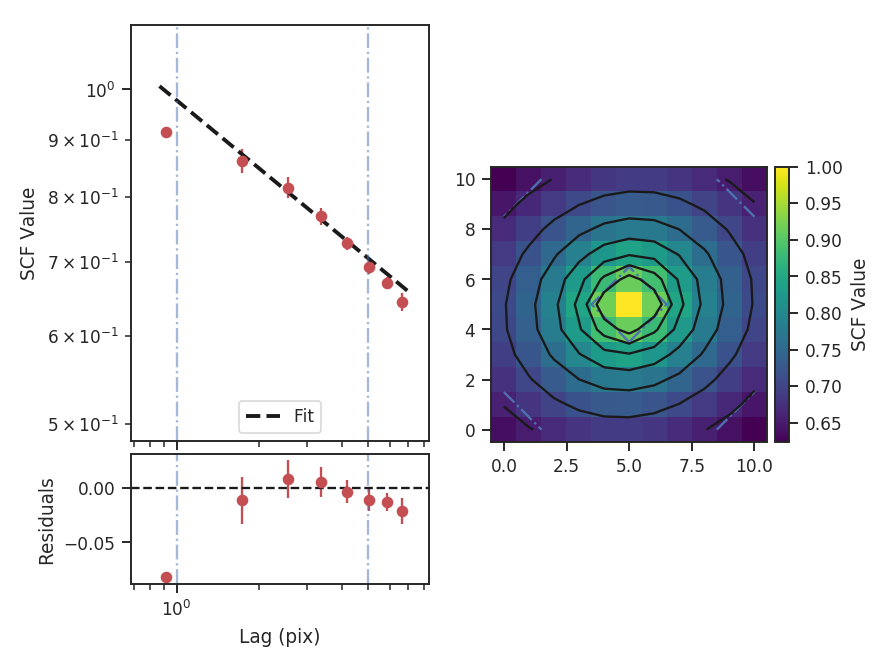
The summary plot shows the correlation surface, a histogram of correlation values, and the 1D spectrum from the azimuthal average, plotted with the power-law fit. A weighted least-squares fit is used to find the slope of the SCF spectrum, where the inverse squared standard deviation from the azimuthal average are used as the weights. The solid contours on the SCF surface are from the 2D fit to the surface, while the blue dot-dashed lines are the extents of the data used in the fit (and match the 1D spectrum limits). See the PowerSpectrum tutorial for a more thorough discussion of the two-dimensional fitting.
The 2D model parameters are not shown in the above summary. Instead, the parameters can be accessed with:
>>> print(scf.slope2D, scf.slope2D_err)  # doctest: +SKIP
(-0.21648274416050342, 0.0029877489213308711)
>>> print(scf.ellip2D, scf.ellip2D_err)  # doctest: +SKIP
(0.89100428375797669, 0.013283231941591638)
>>> print(scf.theta2D, scf.theta2D_err)  # doctest: +SKIP
(0.33117523945671401, 0.06876652735591221)
Since each value in the SCF surface is an average over the whole cube, it tends to be less affected by noise than the power-spectrum based methods (e.g., PowerSpectrum tutorial) and the 2D fit is highly constrained despite having many fewer points to fit. The slope of the 2D model is much steeper than the slope of the 1D model. In the 2D model, the index is defined to be the slope along the minor axis, where the slope is the steepest. The ability to return the slope at any angle will be added to TurbuStat in a future release.
Real data may not have a spectrum described by a single power-law. In this case, the fit limits can be specified using xlow and xhigh to limit which scales are used in the fit.
>>> scf.run(verbose=True, xlow=1 * u.pix, xhigh=5 * u.pix)  # doctest: +SKIP
                            WLS Regression Results
==============================================================================
Dep. Variable:                      y   R-squared:                       0.983
Model:                            WLS   Adj. R-squared:                  0.975
Method:                 Least Squares   F-statistic:                     118.9
Date:                Tue, 18 Jul 2017   Prob (F-statistic):            0.00831
Time:                        10:10:42   Log-Likelihood:                 16.864
No. Observations:                   4   AIC:                            -29.73
Df Residuals:                       2   BIC:                            -30.95
Df Model:                           1
Covariance Type:            nonrobust
==============================================================================
                 coef    std err          t      P>|t|      [0.025      0.975]
------------------------------------------------------------------------------
const         -0.0103      0.010     -1.036      0.409      -0.053       0.032
x1            -0.2027      0.019    -10.902      0.008      -0.283      -0.123
==============================================================================
Omnibus:                          nan   Durbin-Watson:                   2.000
Prob(Omnibus):                    nan   Jarque-Bera (JB):                0.637
Skew:                          -0.020   Prob(JB):                        0.727
Kurtosis:                       1.045   Cond. No.                         10.0
==============================================================================
The one-dimensional power spectrum in the previous examples is averaged over all azimuthal angles. In cases where only a certain range of angles is of interest, limits on the averaged azimuthal angles can be given:
>>> scf.run(verbose=True, xlow=1 * u.pix, xhigh=5 * u.pix,
...         radialavg_kwargs={"theta_0": 1.13 * u.rad,
...                           "delta_theta": 70 * u.deg})  # doctest: +SKIP
                            WLS Regression Results
==============================================================================
Dep. Variable:                      y   R-squared:                       0.987
Model:                            WLS   Adj. R-squared:                  0.981
Method:                 Least Squares   F-statistic:                     157.2
Date:                Mon, 02 Oct 2017   Prob (F-statistic):            0.00630
Time:                        09:00:45   Log-Likelihood:                 17.721
No. Observations:                   4   AIC:                            -31.44
Df Residuals:                       2   BIC:                            -32.67
Df Model:                           1
Covariance Type:            nonrobust
==============================================================================
                 coef    std err          t      P>|t|      [0.025      0.975]
------------------------------------------------------------------------------
const         -0.0067      0.010     -0.695      0.559      -0.048       0.035
x1            -0.2098      0.017    -12.539      0.006      -0.282      -0.138
==============================================================================
Omnibus:                          nan   Durbin-Watson:                   1.899
Prob(Omnibus):                    nan   Jarque-Bera (JB):                0.449
Skew:                          -0.003   Prob(JB):                        0.799
Kurtosis:                       1.358   Cond. No.                         14.4
==============================================================================

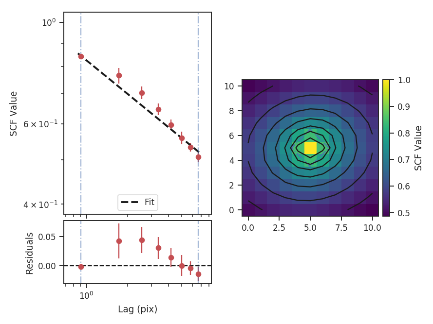
theta_0 is the angle at the center of the azimuthal mask and delta_theta is the width of that mask. The mask is shown on the SCF surface by the radial blue-dashed contours.
Here the fit limits were given in pixel units, but angular units and physical units (if a distance is given) can also be passed. For these data, there is some deviation from a power-law at small lags over the range of lags used and so limiting the fitting range has not significantly changed the fit. See Figure 8 in Padoan et al. 2001 for an example of deviations from power-law behaviour in the SCF spectrum.
The slope of the model can be accessed with scf.slope and its standard error with scf.slope_err. The slope and intercept values are in scf.fit.params. scf.fitted_model can be used to evaluate the model at any given lag value. For example:
>>> scf.fitted_model(1 * u.pix)  # doctest: +SKIP
0.97659777310171636
>>> scf.fitted_model(u.Quantity([1, 10]) * u.pix)  # doctest: +SKIP
array([ 0.97659777,  0.61242384])
>>> scf.fitted_model(u.Quantity([50, 100]) * u.arcsec)  # doctest: +SKIP
array([ 0.44197356,  0.3840506 ])
All values passed must have an attached unit. Physical units can be given when a distance has been given (see below).
In some cases, it may be preferable to calculate the SCF on specific physical scales. When SCF is given a distance,
roll_lags, xlow, xhigh, and xunit can be given in physical units. Angular units can always be given, as well, since SCF requires a FITS header. In this example, we will use a set of custom lags in physical units:
>>> distance = 250 * u.pc  # Assume a distance
>>> phys_conv = (np.abs(cube.header['CDELT2']) * u.deg).to(u.rad).value * distance  # doctest: +SKIP
>>> custom_lags = np.arange(-4.5, 5, 1.5) * phys_conv  # doctest: +SKIP
>>> print(custom_lags)  # doctest: +SKIP
[-0.10296379 -0.06864253 -0.03432126  0.          0.03432126  0.06864253 0.10296379] pc
The lags here are equally spaced and centered around zero. phys_conv converts the pixel values into physical units. When calling SCF, the distance must now be given:
>>> scf_physroll = SCF(cube, roll_lags=custom_lags, distance=distance)  # doctest: +SKIP
>>> scf_physroll.run(verbose=True, xunit=u.pc)  # doctest: +SKIP
                            WLS Regression Results
==============================================================================
Dep. Variable:                      y   R-squared:                       0.892
Model:                            WLS   Adj. R-squared:                  0.856
Method:                 Least Squares   F-statistic:                     24.77
Date:                Tue, 18 Jul 2017   Prob (F-statistic):             0.0156
Time:                        10:57:18   Log-Likelihood:                 14.907
No. Observations:                   5   AIC:                            -25.81
Df Residuals:                       3   BIC:                            -26.59
Df Model:                           1
Covariance Type:            nonrobust
==============================================================================
                 coef    std err          t      P>|t|      [0.025      0.975]
------------------------------------------------------------------------------
const         -0.2522      0.038     -6.725      0.007      -0.372      -0.133
x1            -0.1292      0.026     -4.977      0.016      -0.212      -0.047
==============================================================================
Omnibus:                          nan   Durbin-Watson:                   1.495
Prob(Omnibus):                    nan   Jarque-Bera (JB):                0.757
Skew:                           0.914   Prob(JB):                        0.685
Kurtosis:                       2.464   Cond. No.                         19.3
==============================================================================

This example takes a bit longer to run than the others because, whenever a non-integer lag is used, the cube is shifted in Fourier space.
Throughout all of these examples, we have assumed that the spatial boundaries can be wrapped. This is appropriate for the example data since they are generated from a periodic-box simulation and is the default setting (boundary='continuous'). Typically this will not be the case for observational data. To avoid wrapping the edges of the data, boundary='cut' can be set to avoid using the portion of the data that has been spatially wrapped:
>>> scf = SCF(cube, size=11)  # doctest: +SKIP
>>> scf.run(verbose=True, boundary='cut')  # doctest: +SKIP
                            WLS Regression Results
==============================================================================
Dep. Variable:                      y   R-squared:                       0.993
Model:                            WLS   Adj. R-squared:                  0.992
Method:                 Least Squares   F-statistic:                     830.7
Date:                Tue, 18 Jul 2017   Prob (F-statistic):           1.16e-07
Time:                        11:13:18   Log-Likelihood:                 24.569
No. Observations:                   8   AIC:                            -45.14
Df Residuals:                       6   BIC:                            -44.98
Df Model:                           1
Covariance Type:            nonrobust
==============================================================================
                 coef    std err          t      P>|t|      [0.025      0.975]
------------------------------------------------------------------------------
const         -0.0834      0.003    -31.106      0.000      -0.090      -0.077
x1            -0.2425      0.008    -28.821      0.000      -0.263      -0.222
==============================================================================
Omnibus:                        0.723   Durbin-Watson:                   0.501
Prob(Omnibus):                  0.697   Jarque-Bera (JB):                0.556
Skew:                          -0.236   Prob(JB):                        0.757
Kurtosis:                       1.797   Cond. No.                         3.38
==============================================================================
This results in a steeper SCF slope as the edges of the rolled cubes are no longer used.
Computing the SCF can be computationally expensive for moderately-size data cubes. This is due to the need for shifting the entire cube along the spatial dimensions at each lag value. To avoid recomputing the SCF surface, the results of the SCF can be saved as a pickled object:
>>> scf.save_results(output_name="Design4_SCF", keep_data=False) # doctest: +SKIP
Disabling keep_data will remove the data cube before saving to save storage space.
Having saved the results, they can be reloaded using:
>>> scf = SCF.load_results("Design4_SCF.pkl") # doctest: +SKIP
Note that if keep_data=False was used when saving the file, the loaded version cannot be used to recalculate the SCF.