Spatial Power Spectrum
Overview
A common analysis technique for two-dimensional images is the spatial power spectrum, the square of the 2D Fourier transform of the image. A radial profile of the 2D power spectrum gives the 1D power spectrum. The slope of this 1D spectrum can be compared to the expected indexes in different physical limits. For example, Kolmogorov turbulence follows \(k^{-5/3}\) and Burgers’ turbulence follows \(k^{-2}\) (XXX These need a minus 1, I think? XXX).
Using
The data in this tutorial are available here.
We need to import the PowerSpectrum code, along with a few other common packages:
>>> from turbustat.statistics import PowerSpectrum
>>> from astropy.io import fits
And we load in the data:
>>> moment0 = fits.open("Design4_21_0_0_flatrho_0021_13co.moment0.fits")[0]
The power spectrum is computed using:
>>> pspec = PowerSpectrum(moment0)
>>> pspec.run(verbose=True, ang_units=True, unit=u.arcsec)
                            OLS Regression Results
==============================================================================
Dep. Variable:                      y   R-squared:                       0.971
Model:                            OLS   Adj. R-squared:                  0.970
Method:                 Least Squares   F-statistic:                     1719.
Date:                Tue, 11 Oct 2016   Prob (F-statistic):           1.62e-41
Time:                        18:29:35   Log-Likelihood:                 16.391
No. Observations:                  54   AIC:                            -28.78
Df Residuals:                      52   BIC:                            -24.80
Df Model:                           1
Covariance Type:            nonrobust
==============================================================================
                 coef    std err          t      P>|t|      [95.0% Conf. Int.]
------------------------------------------------------------------------------
const          3.1441      0.065     48.138      0.000         3.013     3.275
x1            -2.5851      0.062    -41.461      0.000        -2.710    -2.460
==============================================================================
Omnibus:                        3.193   Durbin-Watson:                   0.845
Prob(Omnibus):                  0.203   Jarque-Bera (JB):                3.006
Skew:                           0.564   Prob(JB):                        0.222
Kurtosis:                       2.751   Cond. No.                         5.08
==============================================================================
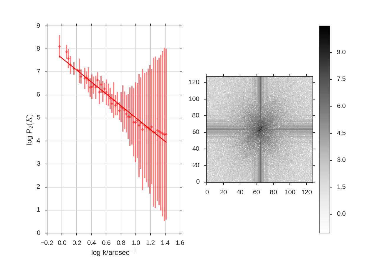
The power spectrum of this simulation has a slope of \(-2.59\pm0.06\). The spatial frequencies (in pixels) used in the fit can be limited by setting low_cut and high_cut. For example,
>>> pspec.run(verbose=True, ang_units=True, unit=u.arcsec, low_cut=0.02, high_cut=0.2)
                            OLS Regression Results
==============================================================================
Dep. Variable:                      y   R-squared:                       0.970
Model:                            OLS   Adj. R-squared:                  0.970
Method:                 Least Squares   F-statistic:                     1148.
Date:                Thu, 27 Oct 2016   Prob (F-statistic):           2.38e-28
Time:                        21:05:20   Log-Likelihood:                 20.760
No. Observations:                  37   AIC:                            -37.52
Df Residuals:                      35   BIC:                            -34.30
Df Model:                           1
Covariance Type:            nonrobust
==============================================================================
                 coef    std err          t      P>|t|      [95.0% Conf. Int.]
------------------------------------------------------------------------------
const          2.7832      0.100     27.781      0.000         2.580     2.987
x1            -2.8618      0.084    -33.883      0.000        -3.033    -2.690
==============================================================================
Omnibus:                        2.438   Durbin-Watson:                   1.706
Prob(Omnibus):                  0.296   Jarque-Bera (JB):                1.614
Skew:                           0.504   Prob(JB):                        0.446
Kurtosis:                       3.180   Cond. No.                         8.59
==============================================================================
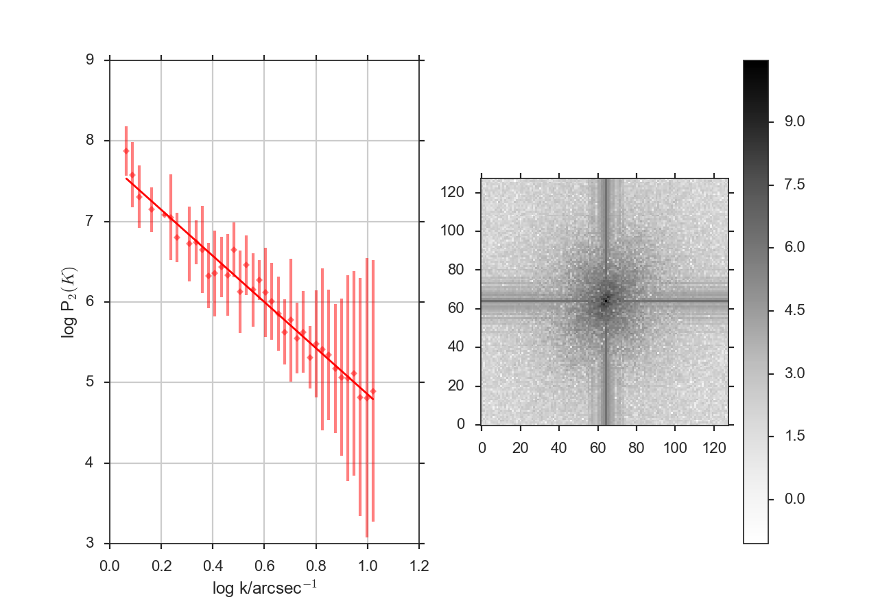
Depending on the inertial range and the noise in the data, you may wish to set limits to recover the correct spatial power spectrum slope. In this case, these limits lead to a steeper slope - \(-2.86\pm0.08\).