Wavelets
Overview
A wavelet transform can be used to filter structure on certain scales, where the scale is typically related to the size and choice of wavelet kernel. By calculating the amount of structure using different sized kernels, the amount of structure on different scales can be calculated. This makes the technique similar to the power-spectrum, but the power at given scale is calculated in the image domain. This approach was introduced for use on astrophysical turbulence by Gill & Henriksen 1990. They used a Mexican-Hat (or Ricker) wavelet for the transform and used the sum of positive values in each filtered map to produce a one-dimensional spectrum between the scale and amount of structure at that scale.
This technique has many similarities to Delta-Variance (see comparison in Zielinsky & Stutzki 1999). Both create a set of filtered maps at different wavelet scales, though the Delta-Variance splits the wavelet kernel into separate component and normalizes by a weight map to reduce edge effects. From the filtered maps, the Delta-Variance measures the variance across the entire map to estimate the amount of structure, while the Wavelet transform assumes the amount of structure is represented by the total of the positive values. From both methods, the slope of the one-dimensional spectrum is the desired measurement.
Using
The data in this tutorial are available here.
We need to import the Wavelet class, along with a few other common packages:
>>> import numpy as np
>>> from turbustat.statistics import Wavelet
>>> from astropy.io import fits
>>> import astropy.units as u
And we load in the data:
>>> moment0 = fits.open("Design4_flatrho_0021_00_radmc_moment0.fits")[0] # doctest: +SKIP
The default wavelet transform of the zeroth moment is calculated as:
>>> wavelet = Wavelet(moment0).run(verbose=True)  # doctest: +SKIP
                            OLS Regression Results
==============================================================================
Dep. Variable:                      y   R-squared:                       0.954
Model:                            OLS   Adj. R-squared:                  0.953
Method:                 Least Squares   F-statistic:                     1001.
Date:                Tue, 01 Aug 2017   Prob (F-statistic):           8.36e-34
Time:                        18:07:44   Log-Likelihood:                 97.550
No. Observations:                  50   AIC:                            -191.1
Df Residuals:                      48   BIC:                            -187.3
Df Model:                           1
Covariance Type:            nonrobust
==============================================================================
                 coef    std err          t      P>|t|      [0.025      0.975]
------------------------------------------------------------------------------
const          1.4175      0.012    119.360      0.000       1.394       1.441
x1             0.3366      0.011     31.635      0.000       0.315       0.358
==============================================================================
Omnibus:                        4.443   Durbin-Watson:                   0.048
Prob(Omnibus):                  0.108   Jarque-Bera (JB):                2.578
Skew:                          -0.334   Prob(JB):                        0.276
Kurtosis:                       2.110   Cond. No.                         4.60
==============================================================================
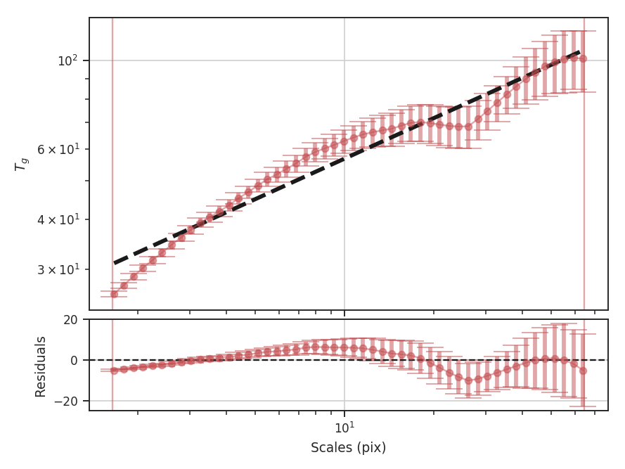
The results of the fit and a plot overlaying the fit on the transform are shown with verbose=True. The figure shows that the transform (blue diamonds) does not follow a single power-law relation across all of the scales and resulting fit (dashed blue line) is poor. The solid blue lines indicate the range of scales used in the fit. In the case of these simulated data, scales larger than about 25 pixels are affected by the edges of the map in the convolution. The flattening on scales just smaller is describing actual features in the data and may be a manifestation of the periodic box conditions; we see a similar feature with these data with the Delta-Variance as well. Unlike the Delta-Variance, the deviation from a power-law is more pronounced on scales larger than about 10 pixels. To improve the fit, we can limit the region that is fit to below this scale:
>>> wavelet = Wavelet(moment0)  # doctest: +SKIP
>>> wavelet.run(verbose=True, xlow=1 * u.pix, xhigh=10 * u.pix)  # doctest: +SKIP
                            OLS Regression Results
==============================================================================
Dep. Variable:                      y   R-squared:                       0.992
Model:                            OLS   Adj. R-squared:                  0.991
Method:                 Least Squares   F-statistic:                     2758.
Date:                Wed, 02 Aug 2017   Prob (F-statistic):           1.86e-25
Time:                        14:05:44   Log-Likelihood:                 78.364
No. Observations:                  25   AIC:                            -152.7
Df Residuals:                      23   BIC:                            -150.3
Df Model:                           1
Covariance Type:            nonrobust
==============================================================================
                 coef    std err          t      P>|t|      [0.025      0.975]
------------------------------------------------------------------------------
const          1.3279      0.006    215.931      0.000       1.315       1.341
x1             0.4946      0.009     52.516      0.000       0.475       0.514
==============================================================================
Omnibus:                        4.021   Durbin-Watson:                   0.122
Prob(Omnibus):                  0.134   Jarque-Bera (JB):                3.476
Skew:                          -0.888   Prob(JB):                        0.176
Kurtosis:                       2.572   Cond. No.                         5.95
==============================================================================
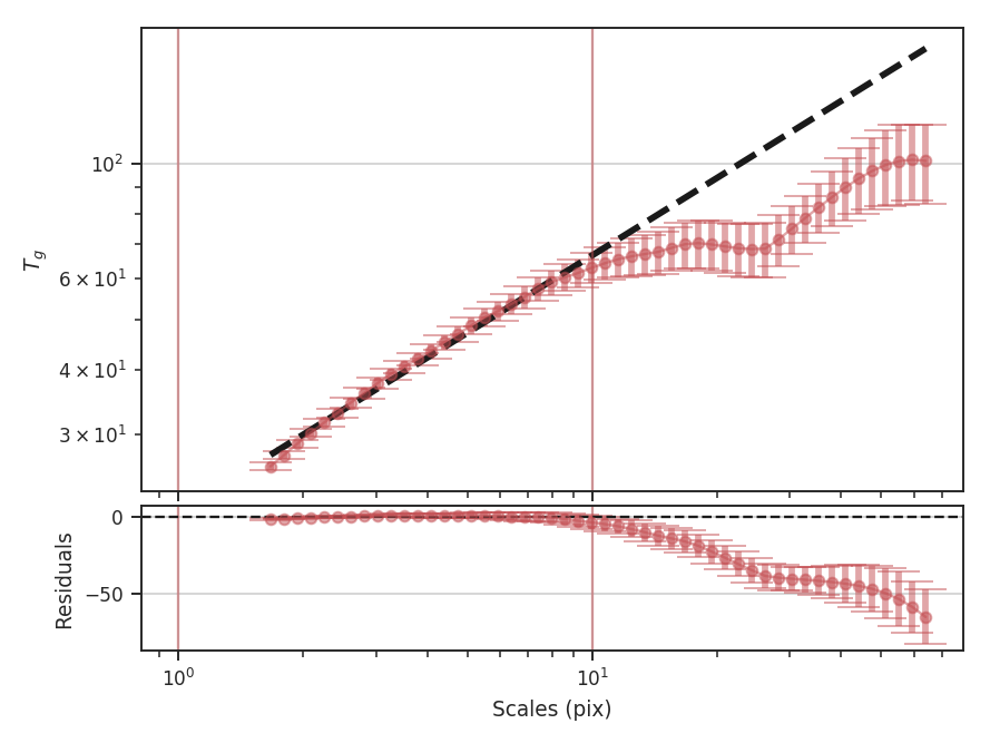
This has significantly improved the fit, and the slope of the power-law is closer to the value found from the Delta-Variance transform. The wavelet transform slope is half of the Delta-Variance slope:
>>> wavelet.slope * 2  # doctest: +SKIP
0.98916576820595215
>>> wavelet.slope_err *2  # doctest: +SKIP
0.018835675570973334
The wavelet transform gives an index of \(0.99 \pm 0.02\), while the Delta-Variance has a slope of \(1.06 \pm 0.02\) fit over a similar range. While limiting the fit gives a consistent result to other methods, the differences in the shape of the spectra may give useful information and should be interpreted carefully.
These examples have used the default scales to calculate the wavelet transforms. The default, in pixel units, will vary from 1.5 pixels to half of the smallest image dimension and will be spaced equally in logarithmic space. The number of scales to test defaults to 50; this can be changed by giving the num keyword to Wavelet. Alternatively, a custom set of scales can be given. The units of the scale can also be given in both angular and physical units (when a distance is provided). This can be useful for comparing different datasets at a common scale. For example, assume that this simulated dataset lies at a distance of 250 pc:
>>> phys_scales = np.arange(0.025, 0.5, 0.05) * u.pc
>>> wavelet = Wavelet(moment0, distance=250 * u.pc, scales=phys_scales)  # doctest: +SKIP
>>> wavelet.run(verbose=True, xlow=1 * u.pix, xhigh=10 * u.pix, xunit=u.pc)  # doctest: +SKIP
                            OLS Regression Results
==============================================================================
Dep. Variable:                      y   R-squared:                       0.983
Model:                            OLS   Adj. R-squared:                  0.977
Method:                 Least Squares   F-statistic:                     173.6
Date:                Wed, 02 Aug 2017   Prob (F-statistic):           0.000944
Time:                        14:43:07   Log-Likelihood:                 11.334
No. Observations:                   5   AIC:                            -18.67
Df Residuals:                       3   BIC:                            -19.45
Df Model:                           1
Covariance Type:            nonrobust
==============================================================================
                 coef    std err          t      P>|t|      [0.025      0.975]
------------------------------------------------------------------------------
const          1.2668      0.031     41.159      0.000       1.169       1.365
x1             0.5649      0.043     13.178      0.001       0.428       0.701
==============================================================================
Omnibus:                          nan   Durbin-Watson:                   1.633
Prob(Omnibus):                    nan   Jarque-Bera (JB):                0.461
Skew:                           0.166   Prob(JB):                        0.794
Kurtosis:                       1.549   Cond. No.                         4.25
==============================================================================
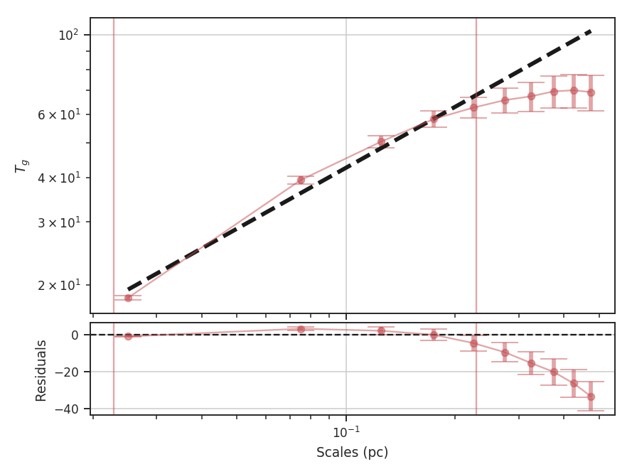
We find a similar slope using the same fit region as the previous example, though with more uncertainty since only 5 of the given scales fit into the region. Note that the plot now shows the scales in parsecs, as well. The output unit used in the plot can be changed by specifying xunit. Similarly, different units can be used in xlow and xhigh, too.
Finally, we note a difference between the TurbuStat implementation of the wavelet transform and the one described in Gill & Henriksen 1990. Their definition of the Mexican-Hat wavelet in Section 2 is an unnormalized form of the kernel and this leads to a slope of \(+2\) larger than the normalized version here. We use the Mexican-Hat implementation from the astropy.convolution package, which has the correct \(1/\pi \sigma^4\) normalization coefficient for the wavelet transform.
The \(+2\) discrepancy can be explained by thinking of the Mexican-Hat kernel as the negative of the Laplacian of a Gaussian. A normalized Gaussian has a normalization constant of \(1/2 \pi \sigma^2\), or units of \(1/{\rm length}^2\), but has a constant peak for all \(\sigma\). In order to make the Laplacian also have a constant peak, referred to as a scale-normalized derivative in image processing, we need to multiply the Mexican-Hat by a factor of \(\sigma^2\) at each scale. Combined with the normalization coefficient of \(1/\pi \sigma^4\), this restores the \(1/{\rm length}^2\) of a Gaussian (Lindeburg 1994). In order to reproduce the unnormalized version of Gill & Henriksen 1990, we need to multiply the kernel by \(\sigma^4\). To reproduce their results, we have included a normalization keyword to disable the correct normalization:
>>> wavelet = Wavelet(moment0)  # doctest: +SKIP
>>> wavelet.run(verbose=True, scale_normalization=False,
...             xhigh=10 * u.pix)  # doctest: +SKIP
                            OLS Regression Results
==============================================================================
Dep. Variable:                      y   R-squared:                       1.000
Model:                            OLS   Adj. R-squared:                  1.000
Method:                 Least Squares   F-statistic:                 7.016e+04
Date:                Wed, 02 Aug 2017   Prob (F-statistic):           1.40e-41
Time:                        15:10:40   Log-Likelihood:                 78.364
No. Observations:                  25   AIC:                            -152.7
Df Residuals:                      23   BIC:                            -150.3
Df Model:                           1
Covariance Type:            nonrobust
==============================================================================
                 coef    std err          t      P>|t|      [0.025      0.975]
------------------------------------------------------------------------------
const          1.3279      0.006    215.931      0.000       1.315       1.341
x1             2.4946      0.009    264.879      0.000       2.475       2.514
==============================================================================
Omnibus:                        4.021   Durbin-Watson:                   0.122
Prob(Omnibus):                  0.134   Jarque-Bera (JB):                3.476
Skew:                          -0.888   Prob(JB):                        0.176
Kurtosis:                       2.572   Cond. No.                         5.95
==============================================================================
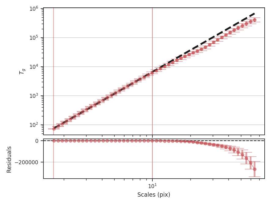
The unnormalized transform appears to follow a power-law relation over all of the scales, and when limited to the same fitting region, the fit appears to be much better. This is deceiving, however, because the extra factors of \(\sigma\) are increasing the correlation between the x and y variables in the fit! This effectively gives a slope of \(+2\) for free, regardless of the data. Further, it means that the fit statistics are no longer valid, as the underlying assumption in the model is that the y and x values are uncorrelated.
Warning
We do not recommend using the unnormalized form as it inflates the quality of the fit, hides the deviations (that may be physically relevant!), but provides no additional information or improvements.