Delta-Variance Distance
See the tutorial for a description of Delta-Variance.
The distance metric for Delta-Variance is DeltaVariance_Distance. There are two definitions of a distance:
- The curve distance is the L2 norm between the delta-variance curves normalized by the sum of each curve:
- \[d_{curve} = \left|\left|\frac{\sigma_{\Delta,1}^2 (\ell)}{\sum_i \sigma_{\Delta,1}^2 (\ell)} - \frac{\sigma_{\Delta,2}^2 (\ell)}{\sum_i \sigma_{\Delta,2}^2 (\ell)}\right|\right|\]
\(\sigma_{\Delta,i}\) are the delta-variance values at lag \(\ell\).
This is a non-parametric attempt to describe the entire delta-variance curve, including regions that are not well fit by a power-law model.
Warning
This distance requires the delta-variance to be measured at the same lags in angular units. This is described further below.
- The slope distance is the t-statistic of the difference in the fitted slopes:
- \[d_{\rm slope} = \frac{|\beta_1 - \beta_2|}{\sqrt{\sigma_{\beta_1}^2 + \sigma_{\beta_1}^2}}\]
\(\beta_i\) are the slopes of the delta-variance curves and \(\sigma_{\beta_i}\) are the uncertainty of the slopes.
More information on the distance metric definitions can be found in Koch et al. 2017
Using
The data in this tutorial are available here.
We need to import the DeltaVariance_Distance class, along with a few other common packages:
>>> from turbustat.statistics import DeltaVariance_Distance
>>> from astropy.io import fits
>>> import matplotlib.pyplot as plt
And we load in the two data sets; in this case, two integrated intensity (zeroth moment) maps:
>>> moment0 = fits.open("Design4_flatrho_0021_00_radmc_moment0.fits")[0]  # doctest: +SKIP
>>> moment0_fid = fits.open("Fiducial0_flatrho_0021_00_radmc_moment0.fits")[0]  # doctest: +SKIP
The error maps are saved in the second extension of these FITS files. These can be used as weights for the Delta-Variance:
>>> moment0_err = fits.open("Design4_flatrho_0021_00_radmc_moment0.fits")[1]  # doctest: +SKIP
>>> moment0_fid_err = fits.open("Fiducial0_flatrho_0021_00_radmc_moment0.fits")[1]  # doctest: +SKIP
The images (and optionally the error maps) are passed to the DeltaVariance_Distance class:
>>> delvar = DeltaVariance_Distance(moment0_fid, moment0, weights1=moment0_err,
...                                weights2=moment0_fid_err)  # doctest: +SKIP
>>> delvar.distance_metric(verbose=True, xunit=u.pix)  # doctest: +SKIP
                            WLS Regression Results
==============================================================================
Dep. Variable:                      y   R-squared:                       0.688
Model:                            WLS   Adj. R-squared:                  0.674
Method:                 Least Squares   F-statistic:                     11.70
Date:                Thu, 01 Nov 2018   Prob (F-statistic):            0.00234
Time:                        13:32:37   Log-Likelihood:                 4.9953
No. Observations:                  25   AIC:                            -5.991
Df Residuals:                      23   BIC:                            -3.553
Df Model:                           1
Covariance Type:                  HC3
==============================================================================
                 coef    std err          z      P>|z|      [0.025      0.975]
------------------------------------------------------------------------------
const          2.5660      0.155     16.602      0.000       2.263       2.869
x1             0.6353      0.186      3.421      0.001       0.271       0.999
==============================================================================
Omnibus:                        3.845   Durbin-Watson:                   0.313
Prob(Omnibus):                  0.146   Jarque-Bera (JB):                3.114
Skew:                          -0.858   Prob(JB):                        0.211
Kurtosis:                       2.784   Cond. No.                         7.05
==============================================================================
                            WLS Regression Results
==============================================================================
Dep. Variable:                      y   R-squared:                       0.956
Model:                            WLS   Adj. R-squared:                  0.954
Method:                 Least Squares   F-statistic:                     66.34
Date:                Thu, 01 Nov 2018   Prob (F-statistic):           3.15e-08
Time:                        13:32:37   Log-Likelihood:                 14.779
No. Observations:                  25   AIC:                            -25.56
Df Residuals:                      23   BIC:                            -23.12
Df Model:                           1
Covariance Type:                  HC3
==============================================================================
                 coef    std err          z      P>|z|      [0.025      0.975]
------------------------------------------------------------------------------
const          1.6490      0.118     14.001      0.000       1.418       1.880
x1             1.3072      0.160      8.145      0.000       0.993       1.622
==============================================================================
Omnibus:                        0.251   Durbin-Watson:                   0.559
Prob(Omnibus):                  0.882   Jarque-Bera (JB):                0.394
Skew:                           0.195   Prob(JB):                        0.821
Kurtosis:                       2.523   Cond. No.                         10.8
==============================================================================
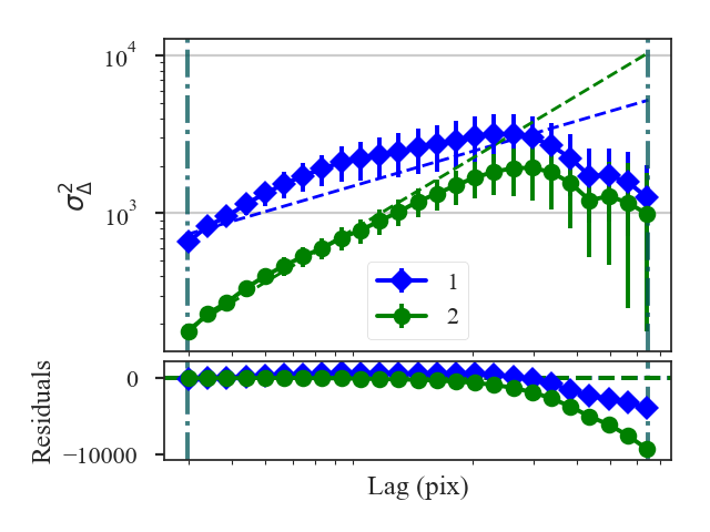
A summary of the fits are printed along with a plot of the two delta-variance curves and the fit residuals when verbose=True. Custom labels can be set by setting label1 and label2 in the distance metric call.
The distances between these two datasets are:
>>> delvar.curve_distance  # doctest: +SKIP
0.8374744762224977
>>> delvar.slope_distance  # doctest: +SKIP
2.737516700717662
In this case, the default settings were used and all portions of the delta-variance curves were used in the fit, yielding poor fits. Setting can be passed to run by specifying inputs to delvar_kwargs. For example, we will now limit the Delta-Variance fitting between 4 and 10 pixel lags:
>>>  delvar_fit = DeltaVariance_Distance(moment0_fid, moment0, weights1=moment0_err,
...                                      weights2=moment0_fid_err,
...                                      delvar_kwargs={'xlow': 4 * u.pix,
...                                                     'xhigh': 10 * u.pix})  # doctest: +SKIP
>>> delvar_fit.distance_metric(verbose=True, xunit=u.pix)  # doctest: +SKIP
                            WLS Regression Results
==============================================================================
Dep. Variable:                      y   R-squared:                       0.985
Model:                            WLS   Adj. R-squared:                  0.982
Method:                 Least Squares   F-statistic:                     77.59
Date:                Thu, 01 Nov 2018   Prob (F-statistic):           0.000313
Time:                        13:32:37   Log-Likelihood:                 20.519
No. Observations:                   7   AIC:                            -37.04
Df Residuals:                       5   BIC:                            -37.15
Df Model:                           1
Covariance Type:                  HC3
==============================================================================
                 coef    std err          z      P>|z|      [0.025      0.975]
------------------------------------------------------------------------------
const          2.4484      0.087     28.186      0.000       2.278       2.619
x1             0.9605      0.109      8.809      0.000       0.747       1.174
==============================================================================
Omnibus:                          nan   Durbin-Watson:                   0.931
Prob(Omnibus):                    nan   Jarque-Bera (JB):                0.657
Skew:                          -0.378   Prob(JB):                        0.720
Kurtosis:                       1.704   Cond. No.                         16.7
==============================================================================
                            WLS Regression Results
==============================================================================
Dep. Variable:                      y   R-squared:                       0.995
Model:                            WLS   Adj. R-squared:                  0.994
Method:                 Least Squares   F-statistic:                     206.3
Date:                Thu, 01 Nov 2018   Prob (F-statistic):           2.95e-05
Time:                        13:32:37   Log-Likelihood:                 23.185
No. Observations:                   7   AIC:                            -42.37
Df Residuals:                       5   BIC:                            -42.48
Df Model:                           1
Covariance Type:                  HC3
==============================================================================
                 coef    std err          z      P>|z|      [0.025      0.975]
------------------------------------------------------------------------------
const          1.7989      0.065     27.823      0.000       1.672       1.926
x1             1.1402      0.079     14.363      0.000       0.985       1.296
==============================================================================
Omnibus:                          nan   Durbin-Watson:                   1.289
Prob(Omnibus):                    nan   Jarque-Bera (JB):                0.654
Skew:                           0.062   Prob(JB):                        0.721
Kurtosis:                       1.507   Cond. No.                         16.6
==============================================================================
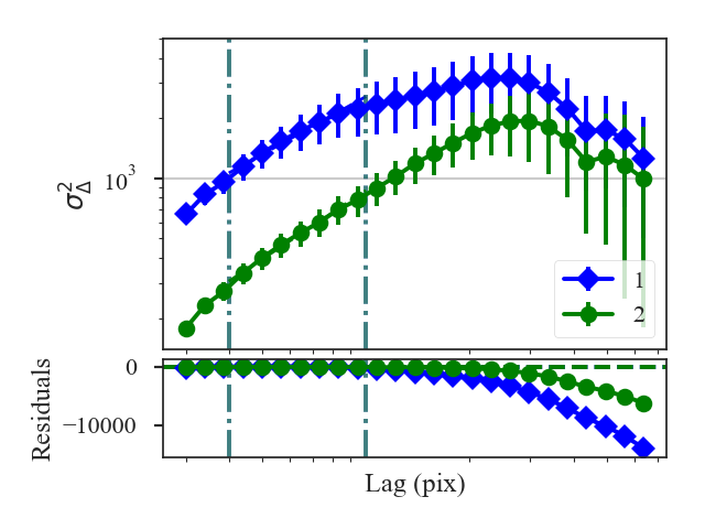
The fits are improved, particularly for the first data set (moment0_fid), with the limits specified. Both of the distances are changed: the slope distance from the improved fits and curve distance because the comparison is limited to the fit limits:
>>> delvar_fit.curve_distance  # doctest: +SKIP
0.06769078224562503
>>> delvar_fit.slope_distance  # doctest: +SKIP
1.3324272202721044
What if you want to set different limits for the two datasets? Or how can you handle datasets with different boundary conditions in the convolution (i.e., observations vs simulated observations)? A second set of kwargs can be given with delvar2_kwargs, which specifies the parameters for the second dataset. For example, to pass a different set of fit limits for the second dataset (moment0):
>>>  delvar_fitdiff = DeltaVariance_Distance(moment0_fid, moment0, weights1=moment0_err,
...                                          weights2=moment0_fid_err,
...                                          delvar_kwargs={'xlow': 4 * u.pix,
...                                                         'xhigh': 10 * u.pix},
...                                          delvar2_kwargs={'xlow': 6 * u.pix,
...                                                          'xhigh': 20 * u.pix})  # doctest: +SKIP
>>> delvar_fitdiff.distance_metric(verbose=True, xunit=u.pix)  # doctest: +SKIP
                            WLS Regression Results
==============================================================================
Dep. Variable:                      y   R-squared:                       0.985
Model:                            WLS   Adj. R-squared:                  0.982
Method:                 Least Squares   F-statistic:                     77.59
Date:                Thu, 01 Nov 2018   Prob (F-statistic):           0.000313
Time:                        13:32:38   Log-Likelihood:                 20.519
No. Observations:                   7   AIC:                            -37.04
Df Residuals:                       5   BIC:                            -37.15
Df Model:                           1
Covariance Type:                  HC3
==============================================================================
                 coef    std err          z      P>|z|      [0.025      0.975]
------------------------------------------------------------------------------
const          2.4484      0.087     28.186      0.000       2.278       2.619
x1             0.9605      0.109      8.809      0.000       0.747       1.174
==============================================================================
Omnibus:                          nan   Durbin-Watson:                   0.931
Prob(Omnibus):                    nan   Jarque-Bera (JB):                0.657
Skew:                          -0.378   Prob(JB):                        0.720
Kurtosis:                       1.704   Cond. No.                         16.7
==============================================================================
                            WLS Regression Results
==============================================================================
Dep. Variable:                      y   R-squared:                       0.999
Model:                            WLS   Adj. R-squared:                  0.999
Method:                 Least Squares   F-statistic:                 1.084e+04
Date:                Thu, 01 Nov 2018   Prob (F-statistic):           1.99e-12
Time:                        13:32:38   Log-Likelihood:                 36.872
No. Observations:                   9   AIC:                            -69.74
Df Residuals:                       7   BIC:                            -69.35
Df Model:                           1
Covariance Type:                  HC3
==============================================================================
                 coef    std err          z      P>|z|      [0.025      0.975]
------------------------------------------------------------------------------
const          1.8957      0.010    198.429      0.000       1.877       1.914
x1             1.0257      0.010    104.110      0.000       1.006       1.045
==============================================================================
Omnibus:                        0.438   Durbin-Watson:                   3.074
Prob(Omnibus):                  0.803   Jarque-Bera (JB):                0.436
Skew:                           0.381   Prob(JB):                        0.804
Kurtosis:                       2.237   Cond. No.                         16.6
==============================================================================
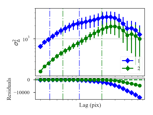
The fit limits, shown with the dot-dashed vertical lines in the plot, differ between the datasets. This will change the slope distance:
>>> delvar_fit.slope_distance  # doctest: +SKIP
0.5956856398497301
But the curve distance is no longer defined:
>>> delvar_fit.curve_distance  # doctest: +SKIP
nan
The curve distance is only valid when the same set of lags are used to compute the delta-variance. Thus having different fit limits violates this condition and the distance is returned as a nan.
The curve distance will also be undefined if different sets of lags are used for the datasets. By default, use_common_lags=True is used in DeltaVariance_Distance, which will find a common set of scales in angular units between the two datasets.
For further fine-tuning of the delta-variance for either dataset, the DeltaVariance classes for each dataset can be accessed as delvar1 and delvar2. Each of these class instances can be run separately, as shown in the delta-variance tutorial, to fine-tune or alter how the delta-variance is computed.