Bispectrum
Overview
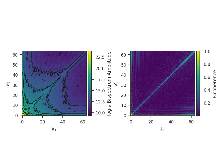
The bispectrum is the Fourier transform of the three-point covariance function. It represents the next higher-order expansion upon the more commonly-used two-point statistics, where the autocorrelation function is the Fourier transform of the power spectrum. The bispectrum is computed using:
where \(\ast\) denotes the complex conjugate, \(F\) is the Fourier transform of some signal, and \(k_1,\,k_2\) are wavenumbers.
The bispectrum retains phase information that is lost in the power spectrum and is therefore useful for investigating phase coherence and coupling.
The use of the bispectrum in the ISM was introduced by Burkhart et al. 2009 and is further used in Burkhart et al. 2010 and Burkhart et al. 2016.
The phase information retained by the bispectrum requires it to be a complex quantity. A real, normalized version can be expressed through the bicoherence. The bicoherence is a measure of phase coupling alone, where the maximal values of 1 and 0 represent complete coupled and uncoupled, respectively. The form that is used here is defined by Hagihira et al. 2001:
The denominator normalizes by the “power” at the modes \(k_1,\,k_2\); this is effectively dividing out the value of the power spectrum, leaving a fractional difference that is entirely the result of the phase coupling. Alternatively, the denominator can be thought of as the value attained if the modes \(k_1\,k_2\) are completely phase coupled, and therefore is the maximal value attainable.
Using
The data in this tutorial are available here.
We need to import the Bispectrum code, along with a few other common packages:
>>> from turbustat.statistics import Bispectrum
>>> from astropy.io import fits
>>> import matplotlib.pyplot as plt
Next, we load in the data:
>>> moment0 = fits.open("Design4_flatrho_0021_00_radmc_moment0.fits")[0] # doctest: +SKIP
While the bispectrum can be extended to sample in N-dimensions, the current implementation requires a 2D input. In all previous work, the computation was performed on an integrated intensity or column density map.
First, the Bispectrum class is initialized:
>>> bispec = Bispectrum(moment0) # doctest: +SKIP
The bispectrum requires only the image, not a header, so passing any arbitrary 2D array will work.
Even using a small 2D image (128x128 here), the number of possible combinations for \(k_1,\,k_2\) is massive (the maximum value of \(k_1,\,k_2\) is half of the largest dimension size in the image). To save time, we can randomly sample some number of phases for each value of \(k_1,\,k_2\) (so \(k_1 + k_2\), the coupling term, changes). This is set by nsamples. There is shot noise associated with this random sampling, and the effect of changing nsamples should be tested. For this example, structure begins to become apparent with about 1000 samples. The figures here use 10000 samples to make the structure more evident. This will take about 10 minutes to run on this image!
The bispectrum and bicoherence maps are computed with run:
>>> bispec.run(verbose=True, nsamples=10000) # doctest: +SKIP
run only performs a single step: compute_bispectrum. For this, there are two optional inputs that may be set:
>>> bispec.run(nsamples=10000, mean_subtract=True, seed=4242424) # doctest: +SKIP
seed sets the random seed for the sampling, and mean_subtract removes the mean from the data before computing the bispectrum. This removes the “zero frequency” power defined based on the largest scale in the image that gives the phase coupling along \(k_1 = k_2\) line. Removing the mean highlights the non-linear mode interactions.
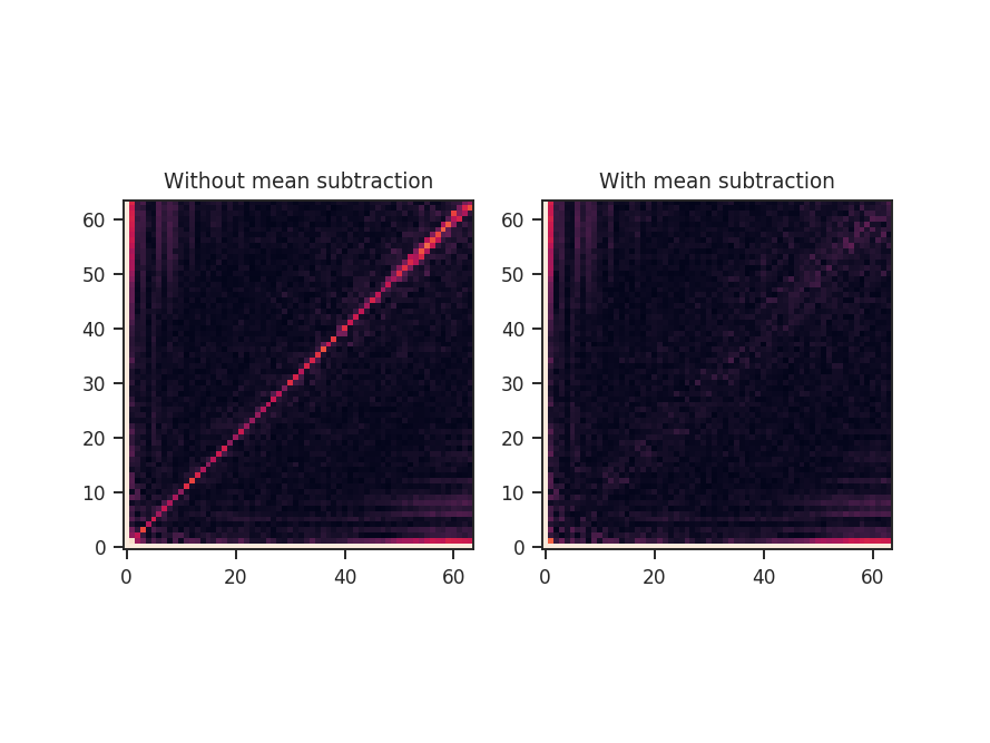
The figure shows the effect on the bicoherence from subtracting the mean. The colorbar is limited between 0 and 1, with black representing 1.
Both radial and azimuthal slices can be extracted from the bispectrum to examine how its properties vary with angle and radius. Using the non-mean subtracted example, radial slices can be returned with:
>>> rad_slices = bispec.radial_slices([30, 45, 60] * u.deg, 20 * u.deg, value='bispectrum_logamp')  # doctest: +SKIP
>>> plt.errorbar(rad_slices[30][0], rad_slices[30][1], yerror=rad_slices[30][2], label='30')  # doctest: +SKIP
>>> plt.errorbar(rad_slices[45][0], rad_slices[45][1], yerror=rad_slices[45][2], label='45')  # doctest: +SKIP
>>> plt.errorbar(rad_slices[60][0], rad_slices[60][1], yerror=rad_slices[60][2], label='60')  # doctest: +SKIP
>>> plt.legend()  # doctest: +SKIP
>>> plt.xlabel("Radius")  # doctest: +SKIP
>>> plt.ylabel("log Bispectrum")  # doctest: +SKIP
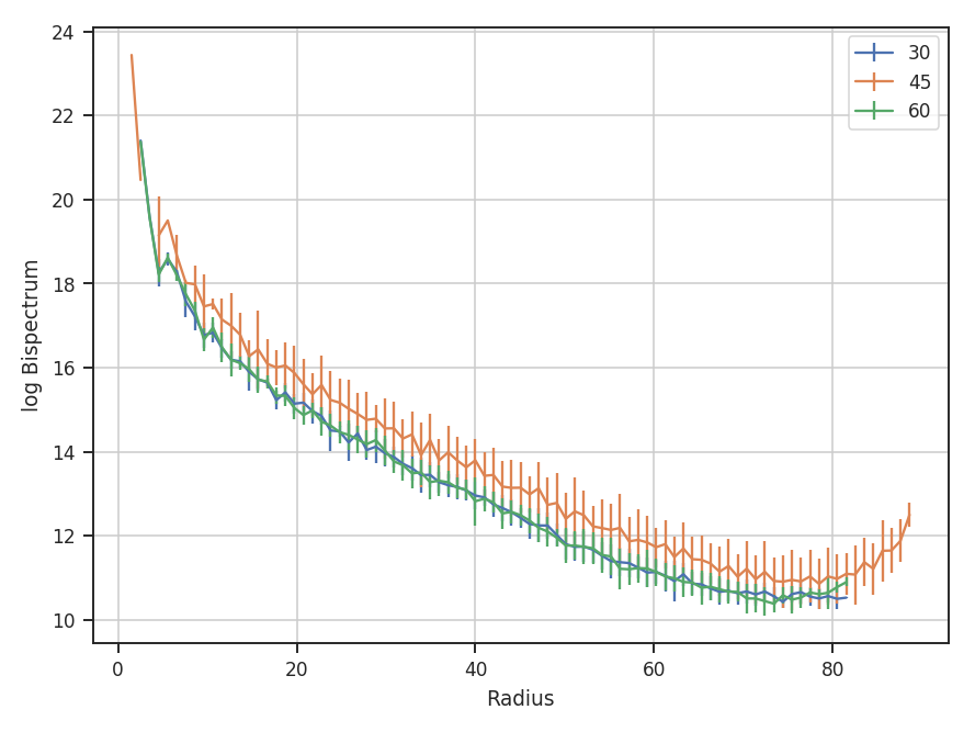
Three slices are returned, centered at 30, 45, and 60 degrees. The width of each slice is 20 degrees. rad_slices is a dictionary whose keys are the (rounded to the nearest integer) center angles given. Each entry in the dictionary has the bin centers ([0]), values ([1]), and standard deviations ([2]). The center angles and slice width can be given in any angular unit. By default, the averaging is over the bispectrum amplitudes. By passing value='bispectrum_logamp', the log of the amplitudes are instead averaged over. The bicoherence array can also be averaged over with value='bicoherence'. The size of the bins can also be changed by passing bin_width to radial_slices; the default is 1.
The azimuthal slices are similarly calculated:
>>> azim_slices = tester.azimuthal_slice([8, 16, 50], 10, value='bispectrum_logamp', bin_width=5 * u.deg)  # doctest: +SKIP
>>> plt.errorbar(azim_slices[8][0], azim_slices[8][1], yerror=azim_slices[8][2], label='8')  # doctest: +SKIP
>>> plt.errorbar(azim_slices[16][0], azim_slices[16][1], yerror=azim_slices[16][2], label='16')  # doctest: +SKIP
>>> plt.errorbar(azim_slices[50][0], azim_slices[50][1], yerror=azim_slices[50][2], label='50')  # doctest: +SKIP
>>> plt.legend()  # doctest: +SKIP
>>> plt.xlabel("Theta (rad)")  # doctest: +SKIP
>>> plt.ylabel("log Bispectrum")  # doctest: +SKIP
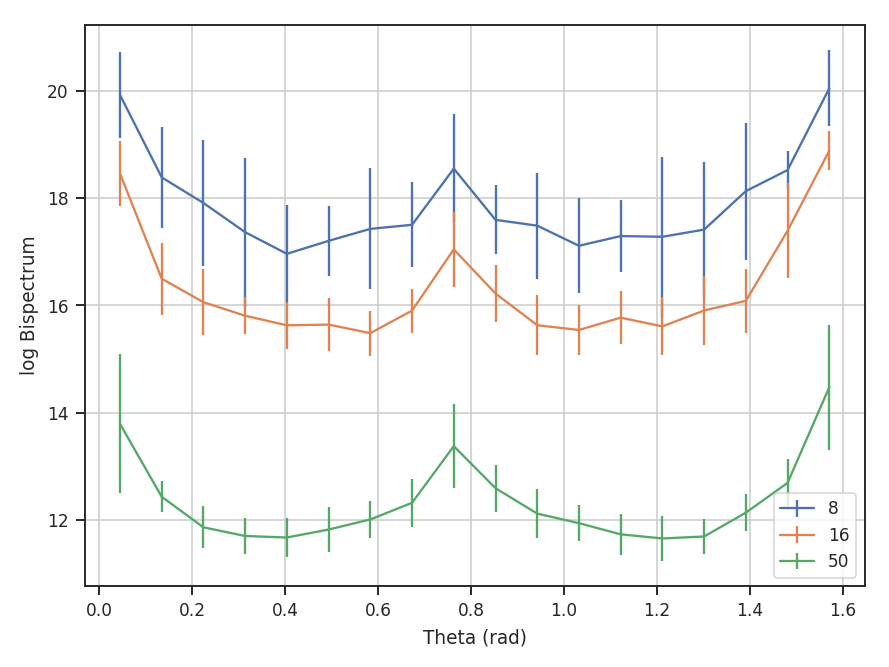
The slices are returned over angles 0 to \(\pi / 2\). With the azimuthal slices, the center radii, in units of the wavevectors, are given and a radial width (10) is specified for all. If different widths are needed, multiple values for the width can be given, though the length must match the length of the center radii.