Dendrograms
Overview
In general, dendrograms provide a hierarchical description of datasets, which may be used to identify clusters of similar objects or variables. This is known as hierarchical clustering. In the case of position-position-velocity (PPV) cubes, a dendrogram is a hierarchical decomposition of the emission in the cube. This decomposition was introduced by Rosolowsky et al. 2008 and Goodman et al. 2009 to calculate the multiscale properties of molecular gas in nearby clouds. The tree structure is comprised of branches and leaves. Branches are the connections, while leaves are the tips of the branches.
Burkhart et al. 2013 introduced two statistics for comparing the dendrograms of two cubes: the relationship between the number of leaves and branches in the tree versus the minimum branch length, and a histogram comparison of the peak intensity in a branch or leaf. The former statistic shows a power-law like turn-off with increasing branch length.
Using
The data in this tutorial are available here.
Requires the optional astrodendro package to be installed. See the documentation
Importing the dendrograms code, along with a few other common packages:
>>> from turbustat.statistics import Dendrogram_Stats
>>> from astropy.io import fits
>>> import astropy.units as u
>>> from astrodendro import Dendrogram
>>> import matplotlib.pyplot as plt
>>> import numpy as np
And we load in the data:
>>> cube = fits.open("Design4_flatrho_0021_00_radmc.fits")[0]
Before running the statistics side, we can first compute the dendrogram itself to see what we’re dealing with:
>>> d = Dendrogram.compute(cube.data, min_value=0.005, min_delta=0.1, min_npix=50, verbose=True)
>>> ax = plt.subplot(111)
>>> d.plotter().plot_tree(ax)
>>> plt.ylabel("Intensity (K)")
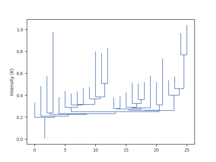
We see a number of leaves of varying height throughout the tree. Their minimum height is set by min_delta. As we increase this value, the tree becomes pruned: more and more structure will be merged, leaving only the brightest regions on the tree.
While this tutorial uses a PPV cube, a 2D image may also be used! The same tutorial code can be used for both, with changes needed for the choice of min_delta.
The statistics are computed through Dendrogram_Stats:
>>> dend_stat = Dendrogram_Stats(cube,
...                              min_deltas=np.logspace(-2, 0, 50),
...                              dendro_params={"min_value": 0.005, "min_npix": 50})
There are two parameters that will change depending on the given data set: (1) min_deltas sets the minimum branch heights, which are completely dependent on the range of values within the data data, and (2) dendro_params, which is a dictionary setting other dendrogram parameters such as the minimum number of pixels a region must have (min_npix) and the minimum values of the data to consider (min_value). The settings given above are specific for these data and will need to be changed when using other data sets.
To run the statistics, we use run:
>>> dend_stat.run(verbose=True)
                            OLS Regression Results
==============================================================================
Dep. Variable:                      y   R-squared:                       0.962
Model:                            OLS   Adj. R-squared:                  0.960
Method:                 Least Squares   F-statistic:                     825.6
Date:                Mon, 03 Jul 2017   Prob (F-statistic):           6.25e-25
Time:                        15:04:02   Log-Likelihood:                 34.027
No. Observations:                  35   AIC:                            -64.05
Df Residuals:                      33   BIC:                            -60.94
Df Model:                           1
Covariance Type:            nonrobust
==============================================================================
                 coef    std err          t      P>|t|      [0.025      0.975]
------------------------------------------------------------------------------
const          0.4835      0.037     13.152      0.000       0.409       0.558
x1            -1.1105      0.039    -28.733      0.000      -1.189      -1.032
==============================================================================
Omnibus:                        4.273   Durbin-Watson:                   0.287
Prob(Omnibus):                  0.118   Jarque-Bera (JB):                3.794
Skew:                          -0.800   Prob(JB):                        0.150
Kurtosis:                       2.800   Cond. No.                         4.39
==============================================================================
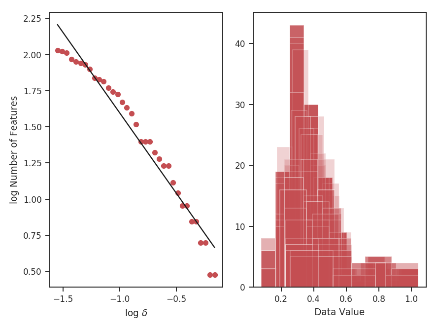
On the left is the relationship between the value of min_delta and the number of features in the tree. On the right is a stack of histograms, showing the distribution of peak intensities for all values of min_delta. The results of the linear fit are also printed, where x1 is the slope of the power-law tail.
When using simulated data from a periodic box, the boundaries need to be handled across the edges. Setting periodic_bounds=True will treat the spatial dimensions as periodic. The simulated data shown here should have periodic_bounds enabled:
>>> dend_stat.run(verbose=True, periodic_bounds=True)
                            OLS Regression Results
==============================================================================
Dep. Variable:                      y   R-squared:                       0.962
Model:                            OLS   Adj. R-squared:                  0.961
Method:                 Least Squares   F-statistic:                     808.6
Date:                Thu, 06 Jul 2017   Prob (F-statistic):           2.77e-24
Time:                        13:30:48   Log-Likelihood:                 33.415
No. Observations:                  34   AIC:                            -62.83
Df Residuals:                      32   BIC:                            -59.78
Df Model:                           1
Covariance Type:            nonrobust
==============================================================================
                 coef    std err          t      P>|t|      [0.025      0.975]
------------------------------------------------------------------------------
const          0.3758      0.039      9.744      0.000       0.297       0.454
x1            -1.1369      0.040    -28.437      0.000      -1.218      -1.055
==============================================================================
Omnibus:                        4.386   Durbin-Watson:                   0.267
Prob(Omnibus):                  0.112   Jarque-Bera (JB):                4.055
Skew:                          -0.823   Prob(JB):                        0.132
Kurtosis:                       2.611   Cond. No.                         4.60
==============================================================================
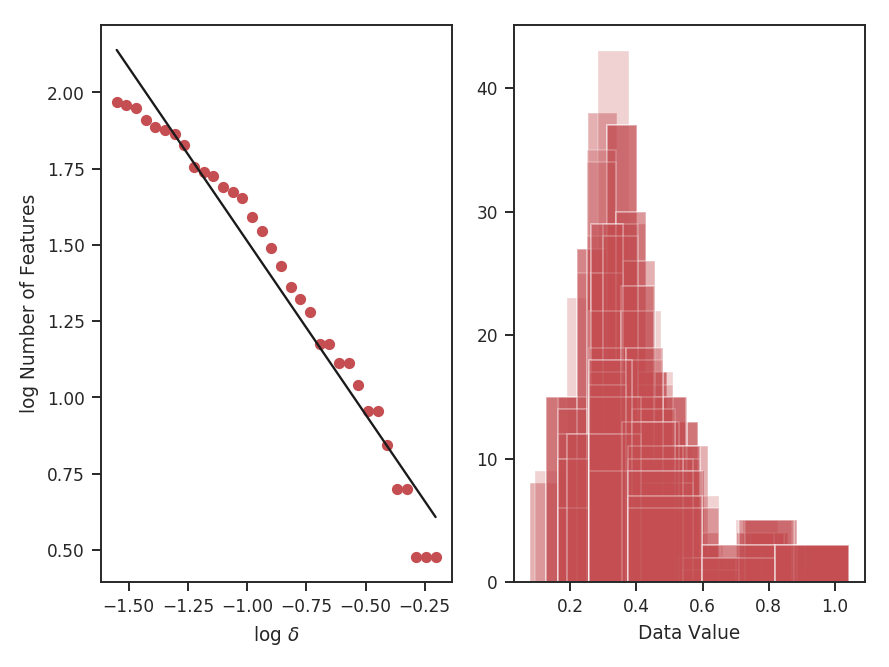
The results have slightly changed. The left panel shows fewer features at nearly every value of \(\delta\) as regions along the edges are connected across the boundaries.
Creating the initial dendrogram is the most time-consuming step. To check the progress of building the dendrogram, dendro_verbose=True can be set in the previous call to give a progress bar and time-to-completion estimate.
Computing dendrograms can be time-consuming when working with large datasets. We can avoid recomputing a dendrogram by loading from an HDF5 file:
>>> dend_stat = Dendrogram_Stats.load_dendrogram("design4_dendrogram.hdf5",
...                                              min_deltas=np.logspace(-2, 0, 50))
Saving the dendrogram structure is explained in the astrodendro documentation. The saved dendrogram must have min_delta set to the minimum of the given min_deltas. Otherwise pruning is ineffective.
If the dendrogram is stored in a variable (say you have just run it in the same terminal), you may pass the computed dendrogram into run:
>>> d = Dendrogram.compute(cube, min_value=0.005, min_delta=0.01, min_npix=50, verbose=True)
>>> dend_stat = Dendrogram_Stats(cube, min_deltas=np.logspace(-2, 0, 50))
>>> dend_stat.run(verbose=True, dendro_obj=d)
Once the statistics have been run, the results can be saved as a pickle file:
>>> dend_stat.save_results(output_name="Design4_Dendrogram_Stats.pkl", keep_data=False)
keep_data=False will avoid saving the entire cube and is the default setting.
Saving can also be enabled with run:
>>> dend_stat.run(save_results=True, output_name="Design4_Dendrogram_Stats.pkl")
The results may then be reloaded:
>>> dend_stat = Dendrogram_Stats.load_results("Design4_Dendrogram_Stats.pkl")
Note that the dendrogram and data are NOT saved, and only the statistic outputs will be accessible.