Bispectrum
Overview
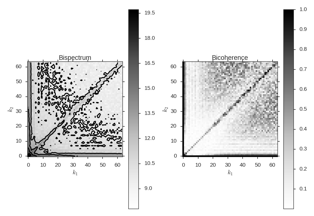
The bispectrum is the Fourier transform of the three-point covariance function. It represents the next higher-order expansion upon the more commonly used two-point statistics, whose autocorrelation function is the power spectrum. The bispectrum is computed using:
where \(\ast\) denotes the complex conjugate, \(F\) is the Fourier transform of some signal, and \(k_1,\,k_2\) are wavenumbers.
The bispectrum retains phase information which is lost in the power spectrum, and is therefore useful for investigating phase coherence and coupling.
The use of the bispectrum in the ISM was introduced by Burkhart et al. 2009, and recently extended in Burkhart et al. 2016.
The phase information retained by the bispectrum requires it to be a complex quantity. A real, normalized version can be expressed through the bicoherence. The bicoherence is a measure of phase coupling alone, where the maximal values of 1 and 0 represent complete coupled and uncoupled, respectively. The form that is used here is defined by Hagihira et al. 2001:
The denominator normalizes out the “power” at the modes \(k_1,\,k_2\); this is effectively dividing out the value of the power spectrum, leaving a fractional difference that is entirely the result of the phase coupling. Alternatively, the denominator can be thought of as the value attained if the modes \(k_1\,k_2\) are completely phase coupled, and therefore is the maximal value attainable.
In the recent work of Burkhart et al. 2016, they used a phase coherence technique (PCI), alternative to the bispectrum, to measure phase coherence as a function of radial and azimuthal changes (so called lags averaged over radius or angle in the bispectrum plane). This is defined as
where \(L(R)\) is the relevant averaged quantity calculated at different lags (denoted generally by \(R\)). ORG is the original signal, PRS is the signal with randomized phases, and PCS is the signal with phases set to be correlated. For each value of R, this yields a normalized value (\(C(R)\)) between 0 and 1, similar to the bispectrum. Note: PCI will be added to the existing TurbuStat code, but is not yet complete..
Using
The data in this tutorial are available here.
We need to import the BiSpectrum code, along with a few other common packages:
>>> from turbustat.statistics import BiSpectrum
>>> from astropy.io import fits
And we load in the data:
>>> moment0 = fits.open("Design4_21_0_0_flatrho_0021_13co.moment0.fits")[0]
While the bispectrum can be extended to sample in N-dimensions, the current implementation requires a 2D input. In all previous work, the computation is performed on an integrated intensity or column density map.
First, the BiSpectrum class is initialized:
>>> bispec = BiSpectrum(moment0)
The bispectrum requires only the image, not a header, so passing any arbitrary 2D array will work.
The entire computation is performed through run:
>>> bispec.run(verbose=True, nsamples=1.e3)
Even in small 2D image (128x128 here), the number of possible combinations for \(k_1,\,k_2\) is already massive (the maximum value of \(k_1,\,k_2\) is half of the largest dimension size in the image). To minimize the computational time, we can randomly sample some number of phases for each value of \(k_1,\,k_2\) (so \(k_1 + k_2\), the coupling term, changes). This is set by nsamples. There is shot noise associated with this random sampling, and so different nsamples should be tested. In this, structure begins to become more apparent with around 1000, and improves beyond this (at the expense of time).
run is really only hiding a single step: compute_bispectrum. There are two additional inputs which may be set:
>>> bispec.run(nsamples=1.e3, mean_subtract=True, seed=4242424)
The two additional arguments here are seed, to set the random seed for sampling, and mean_subtract, which first removes the mean from the data before computing the bispectrum. The removes the “zero frequency” power defined based on the largest scale in the image and removes much the phase coupling along the \(k_1 = k_2\) line, highlighting the non-linear mode interactions:
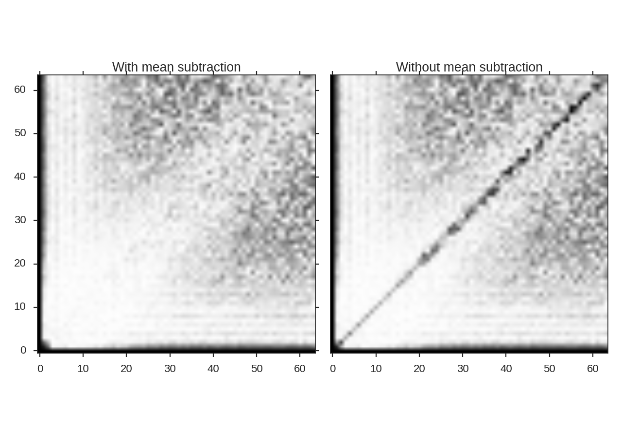
The figure shows the effect on the bicoherence from subtracting the mean. The colorbar is limited between 0 and 1, with black representing 1.