Delta-Variance
Overview
The \(\Delta\)-variance technique was introduced by Stutzki et al. 1998 as a generalization of Allan-variance, a technique used to study the drift in instrumentation. They found that molecular cloud structures are well characterized by fractional Brownian motion structure, which results from a power-law power spectrum with a random phase distribution. The technique was extended by Bensch et al. 2001 to account for the effects of beam smoothing and edge effects on a discretely sampled grid. With this, they identified a functional form to recover the index of the near power-law relation. The technique was extended again by Ossenkopf et al. 2008a, where the computation using filters of different scales was moved in to the Fourier domain, allowing for a significant improvement in speed. The following description uses their formulation.
Delta-variance measures the amount of structure on a given range of scales. Each delta-variance point is calculated by filtering an image with a spherically symmetric kernel - a French-hat or Mexican hat (Ricker) kernels - and computing the variance of the filtered map. Due to the effects of a finite grid that typically does not have periodic boundaries and the effects of noise, Ossenkopf et al. 2008a proposed a convolution based method that splits the kernel into its central peak and outer annulus, convolves the separate regions, and subtracts the annulus-convolved map from the peak-convolved map. The Mexican-hat kernel separation can be defined using two Gaussian functions. A weight map was also introduced to minimize noise effects where there is low S/N regions in the data. Altogether, this is expressed as:
where \(r\) is the kernel size, \(G\) is the convolved image map, and \(W\) is the convolved weight map. The delta-variance is then,
where \(W_{\rm tot}(r) = W_{\rm core}(r)\,W_{\rm ann}(r)\).
Since the kernel is separated into two components, the ratio between their widths can be set independently. Ossenkopf et al. 2008a find an optimal ratio of 1.5 for the Mexican-hat kernel, which is the element used in TurbuStat.
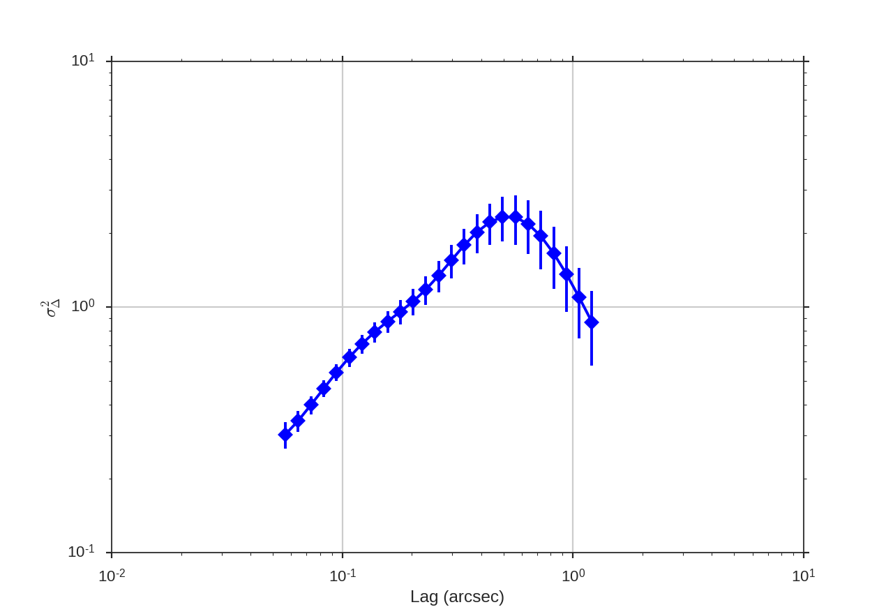
Performing this operation yields a power-law-like relation between the scales \(r\) and the delta-variance.
Using
The data in this tutorial are available here.
We need to import the DeltaVariance code, along with a few other common packages:
>>> from turbustat.statistics import DeltaVariance
>>> from astropy.io import fits
Then, we load in the data and the associated error array:
>>> moment0 = fits.open("Design4_21_0_0_flatrho_0021_13co.moment0.fits")[0]
>>> moment0_err = fits.open("Design4_21_0_0_flatrho_0021_13co.moment0_error.fits")[0]
Next, we initialize the DeltaVariance class:
>>> delvar = DeltaVariance(moment0, weights=moment0_err)
The weight array is optional, but is recommended. Note that this is not the exact form of a weight array used by Ossenkopf et al. 2008b, who used the sqrt of the number of elements along the line of sight used to create the integrated intensity map. This doesn’t take into account the varying S/N of each element used, however. In the case with the simulated data, the two are nearly identical, since the noise value associated with each element is constant. If no weights are given, a uniform array of ones is used.
By default, 25 lag values will be used, logarithmically spaced between 3 pixels to half of the minimum axis size. Alternative lags can be specified by setting the lags keyword. If a ndarray is passed, it is assumed to be in pixel units. Lags can also be given in angular units.
The entire process is performed through run:
>>> delvar.run(verbose=True, ang_units=True, unit=u.arcmin)
ang_units sets showing angular scales in the plot, and unit is the unit to show them in.