Wavelet Distance
See the tutorial for a description of Delta-Variance.
The distance metric for wavelets is Wavelet_Distance. The distance is defined as the t-statistic of the difference between the slopes of the wavelet transforms:
\(\beta_i\) are the slopes of the wavelet transforms and \(\sigma_{\beta_i}\) are the uncertainty of the slopes.
More information on the distance metric definitions can be found in Koch et al. 2017
Using
The data in this tutorial are available here.
We need to import the Wavelet_Distance class, along with a few other common packages:
>>> from turbustat.statistics import Wavelet
>>> from astropy.io import fits
>>> import matplotlib.pyplot as plt
>>> import astropy.units as u
And we load in the two data sets; in this case, two integrated intensity (zeroth moment) maps:
>>> moment0 = fits.open("Design4_flatrho_0021_00_radmc_moment0.fits")[0]  # doctest: +SKIP
>>> moment0_fid = fits.open("Fiducial0_flatrho_0021_00_radmc_moment0.fits")[0]  # doctest: +SKIP
The two images are input to Wavelet_Distance:
>>> wavelet = Wavelet_Distance(moment0_fid, moment0, xlow=2 * u.pix,
...                            xhigh=10 * u.pix)  # doctest: +SKIP
This call will run Wavelet on both of the images, which can be accessed with wt1 and wt2.
In this example, we have limited the fitting regions with xlow and xhigh. Separate fitting limits for each image can be given by giving a two-element list for either keywords (e.g., xlow=[1 * u.pix, 2 * u.pix]). Additional fitting keyword arguments can be passed with fit_kwargs and fit_kwargs2 for the first and second images, respectively.
To calculate the distance:
>>> delvar.distance_metric(verbose=True, xunit=u.pix)  # doctest: +SKIP
                       OLS Regression Results
==============================================================================
Dep. Variable:                      y   R-squared:                       0.983
Model:                            OLS   Adj. R-squared:                  0.982
Method:                 Least Squares   F-statistic:                     1013.
Date:                Fri, 16 Nov 2018   Prob (F-statistic):           1.31e-18
Time:                        17:55:59   Log-Likelihood:                 73.769
No. Observations:                  22   AIC:                            -143.5
Df Residuals:                      20   BIC:                            -141.4
Df Model:                           1
Covariance Type:                  HC3
==============================================================================
                 coef    std err          z      P>|z|      [0.025      0.975]
------------------------------------------------------------------------------
const          1.5636      0.006    267.390      0.000       1.552       1.575
x1             0.3137      0.010     31.832      0.000       0.294       0.333
==============================================================================
Omnibus:                        3.421   Durbin-Watson:                   0.195
Prob(Omnibus):                  0.181   Jarque-Bera (JB):                1.761
Skew:                          -0.397   Prob(JB):                        0.414
Kurtosis:                       1.864   Cond. No.                         7.05
==============================================================================
                            OLS Regression Results
==============================================================================
Dep. Variable:                      y   R-squared:                       0.993
Model:                            OLS   Adj. R-squared:                  0.993
Method:                 Least Squares   F-statistic:                     1351.
Date:                Fri, 16 Nov 2018   Prob (F-statistic):           7.76e-20
Time:                        17:55:59   Log-Likelihood:                 75.406
No. Observations:                  22   AIC:                            -146.8
Df Residuals:                      20   BIC:                            -144.6
Df Model:                           1
Covariance Type:                  HC3
==============================================================================
                 coef    std err          z      P>|z|      [0.025      0.975]
------------------------------------------------------------------------------
const          1.3444      0.008    158.895      0.000       1.328       1.361
x1             0.4728      0.013     36.752      0.000       0.448       0.498
==============================================================================
Omnibus:                        4.214   Durbin-Watson:                   0.170
Prob(Omnibus):                  0.122   Jarque-Bera (JB):                3.493
Skew:                          -0.958   Prob(JB):                        0.174
Kurtosis:                       2.626   Cond. No.                         7.05
==============================================================================
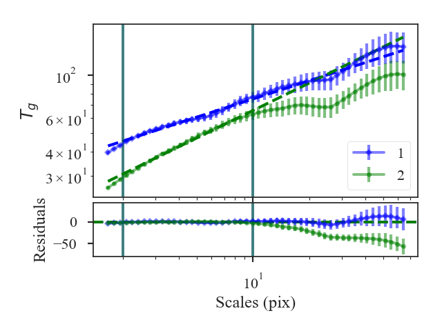
A summary of the fits are printed along with a plot of the two wavelet transforms and the fit residuals. Colours, labels, and symbols can be specified in the plot with plot_kwargs1 and plot_kwargs2.
The distances between these two datasets are:
>>> wavelet.curve_distance  # doctest: +SKIP
9.81949754947785
A pre-computed Wavelet class can be also passed instead of a data cube. See the distance metric introduction.