Bispectrum Distance
See the tutorial for a description of the bispectrum.
The distance metric for the bispectrum is Bispectrum_Distance. There are two definitions of a distance:
- The surface distance is the L2 norm between the bicoherence surfaces of two 2D images:
- \[d_{\rm surface} = ||b_1(k_1, k_2) - b_2(k_1, k_2)||^2\]
The \(k_1,\,k_2\) are wavenumbers and \(b_1,\,b_2\) are the bicoherence arrays for each image.
Warning
The images must have the same shape to use this definition of distance.
- The mean distance is the absolute difference between the mean bicoherence of two 2D images:
- \[d_{\rm mean} = |\bar{b_1(k_1, k_2)} - \bar{b_1(k_1, k_2)}|\]
This distance metric can be used with images of different shapes.
The bicoherence surface is used for the distance metric because it is normalized between 0 and 1, and this normalization removes the effect of the mean of the images (meansub in the bispectrum tutorial).
More information on the distance metric definitions can be found in Koch et al. 2017
Using
The data in this tutorial are available here.
We need to import the Bispectrum_Distance class, along with a few other common packages:
>>> from turbustat.statistics import Bispectrum_Distance
>>> from astropy.io import fits
>>> import matplotlib.pyplot as plt
And we load in the two data sets; in this case, two integrated intensity (zeroth moment) maps:
>>> moment0 = fits.open("Design4_flatrho_0021_00_radmc_moment0.fits")[0]  # doctest: +SKIP
>>> moment0_fid = fits.open("Fiducial0_flatrho_0021_00_radmc_moment0.fits")[0]  # doctest: +SKIP
The images are passed to the Bispectrum_Distance class. Keyword arguments to run can also be given as the dictionary stat_kwargs. In this case, we will increase the number of random samples used to estimate the bispectrum:
>>> bispec = Bispectrum_Distance(moment0_fid, moment0,
...                              stat_kwargs={'nsamples': 10000})  # doctest: +SKIP
This call executes run for both images and may take a few minutes to run (reduce the number of samples to speed things up). Within Bispectrum_Distance is a Bispectrum for each image: bispec1 and bispec2. Each of these class instances can be run separately with, as shown in the bispectrum tutorial, to fine-tune or alter how the bispectrum is computed.
Once the bispectra are computed, we can calculate the distances between the two bispectra and create a summary plot with:
>>> bispec.distance_metric(verbose=True) # doctest: +SKIP
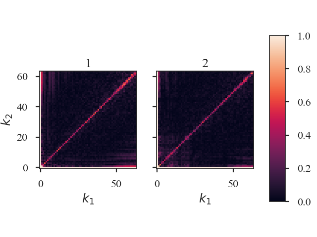
The bicoherence surfaces of both images are shown. By default, the plots are labelled with “1” and “2” in the order the data were given to Bispectrum_Distance. Custom labels can be set by setting label1 and label2 in the distance metric call.
The distances between these images are:
>>> bispec.surface_distance  # doctest: +SKIP
3.169320958026329
Since these images have equal shapes,
surface_distanceis defined. If the images do not have equal shapes, the distance will beNaN.>>> bispec.mean_distance # doctest: +SKIP 0.009241794373870557
Warning
Caution must be used when passing a pre-computed Bispectrum instead of the data for moment0 or moment0_fid as there are no checks to ensure the bispectra were computed the same way (e.g., do both have mean_sub=True set?). Ensure that the keyword arguments for the pre-computed statistic match those specified to Bispectrum_Distance. See the distance metric introduction.