PCA Distance
See the tutorial for a description of Principal Component Analysis (PCA).
We define the PCA distance as the L2 distance between the normalized eigenvalues of two spectral-line data cubes:
The normalized eigenvalues are \(\lambda_{i} / \sum_i \lambda_{i}\).
More information on the distance metric definitions can be found in Koch et al. 2017.
Using
The data in this tutorial are available here.
We need to import the PCA_Distance class, along with a few other common packages:
>>> from turbustat.statistics import PCA_Distance
>>> from astropy.io import fits
>>> import matplotlib.pyplot as plt
PCA_Distance takes two data cubes as input:
>>> cube = fits.open("Design4_flatrho_0021_00_radmc.fits")[0]  # doctest: +SKIP
>>> cube_fid = fits.open("Fiducial0_flatrho_0021_00_radmc.fits")[0]  # doctest: +SKIP
>>> pca = PCA_Distance(cube_fid, cube, n_eigs=50, mean_sub=True)  # doctest: +SKIP
There are two additional keywords that set the number of eigenvalues to include in the distance calculation (n_eigs), and whether to subtract the mean from each spectral channel (mean_sub).
To calculate the distance between the eigenvalues:
>>> pca.distance_metric(verbose=True)  # doctest: +SKIP
Proportions of total variance: 1 - 1.000, 2 - 1.000
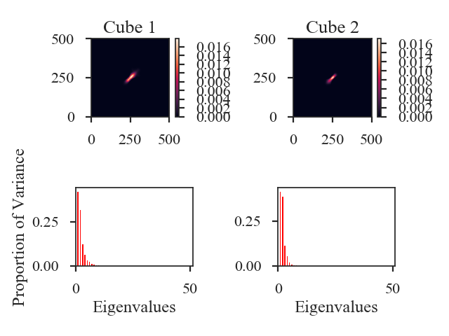
This prints out what fraction of the total variance is included in the eigenvalue vectors for each data cube. The image shows the covariance matrix for each data cube in the first row and a bar chart of the eigenvalues in the second row.
And the distance is:
>>> pca.distance  # doctest: +SKIP
0.07211706060387167
Note that a comparison of the size-line width from PCA as a distance metric is not yet implemented.
A pre-computed PCA class can also be passed instead of a dataset. See the distance metric introduction.