Spatial Power Spectrum Distance
See the tutorial for a description of the spatial power-spectrum.
The distance metric for the power-spectrum is PSpec_Distance. The distance is defined as the t-statistic between the indices of the power-spectra:
\(\beta_i\) are the slopes of the power-spectra and \(\sigma_{\beta_i}\) are the uncertainties.
More information on the distance metric definitions can be found in Koch et al. 2017
Using
The data in this tutorial are available here.
We need to import the Pspec_Distance class, along with a few other common packages:
>>> from turbustat.statistics import PSpec_Distance
>>> from astropy.io import fits
>>> import matplotlib.pyplot as plt
>>> import astropy.units as u
And we load in the two data sets; in this case, two integrated intensity (zeroth moment) maps:
>>> moment0 = fits.open("Design4_flatrho_0021_00_radmc_moment0.fits")[0]  # doctest: +SKIP
>>> moment0_fid = fits.open("Fiducial0_flatrho_0021_00_radmc_moment0.fits")[0]  # doctest: +SKIP
These two images are given as inputs to Pspec_Distance. We know from the power-spectrum tutorial that there should be limits set on where the power-spectra are fit. These can be specified with low_cut and high_cut, along with breaks if the power-spectrum is best fit with a broken power-law model. In this case, we will use the same fit limits for both power-spectra, but separate limits can be given for each image by giving a two-element list to any of these three keywords.
>>> pspec = PSpec_Distance(moment0_fid, moment0,
...                        low_cut=0.025 / u.pix, high_cut=0.1 / u.pix,)  # doctest: +SKIP
This will create and run two PowerSpectrum instances, which can be accessed as pspec1 and pspec2.
To find the distance between these two images, we run:
>>> pspec.distance_metric(verbose=True, xunit=u.pix**-1)  # doctest: +SKIP
                            OLS Regression Results
==============================================================================
Dep. Variable:                      y   R-squared:                       0.930
Model:                            OLS   Adj. R-squared:                  0.924
Method:                 Least Squares   F-statistic:                     222.2
Date:                Wed, 14 Nov 2018   Prob (F-statistic):           4.18e-09
Time:                        10:21:04   Log-Likelihood:                 11.044
No. Observations:                  14   AIC:                            -18.09
Df Residuals:                      12   BIC:                            -16.81
Df Model:                           1
Covariance Type:                  HC3
==============================================================================
                 coef    std err          z      P>|z|      [0.025      0.975]
------------------------------------------------------------------------------
const          6.8004      0.202     33.648      0.000       6.404       7.197
x1            -2.3745      0.159    -14.905      0.000      -2.687      -2.062
==============================================================================
Omnibus:                        0.495   Durbin-Watson:                   2.400
Prob(Omnibus):                  0.781   Jarque-Bera (JB):                0.547
Skew:                          -0.148   Prob(JB):                        0.761
Kurtosis:                       2.078   Cond. No.                         15.2
==============================================================================
                            OLS Regression Results
==============================================================================
Dep. Variable:                      y   R-squared:                       0.971
Model:                            OLS   Adj. R-squared:                  0.968
Method:                 Least Squares   F-statistic:                     495.9
Date:                Wed, 14 Nov 2018   Prob (F-statistic):           3.96e-11
Time:                        10:21:04   Log-Likelihood:                 14.077
No. Observations:                  14   AIC:                            -24.15
Df Residuals:                      12   BIC:                            -22.87
Df Model:                           1
Covariance Type:                  HC3
==============================================================================
                 coef    std err          z      P>|z|      [0.025      0.975]
------------------------------------------------------------------------------
const          5.5109      0.171     32.289      0.000       5.176       5.845
x1            -3.0223      0.136    -22.269      0.000      -3.288      -2.756
==============================================================================
Omnibus:                        0.901   Durbin-Watson:                   2.407
Prob(Omnibus):                  0.637   Jarque-Bera (JB):                0.718
Skew:                          -0.215   Prob(JB):                        0.698
Kurtosis:                       1.977   Cond. No.                         15.2
==============================================================================
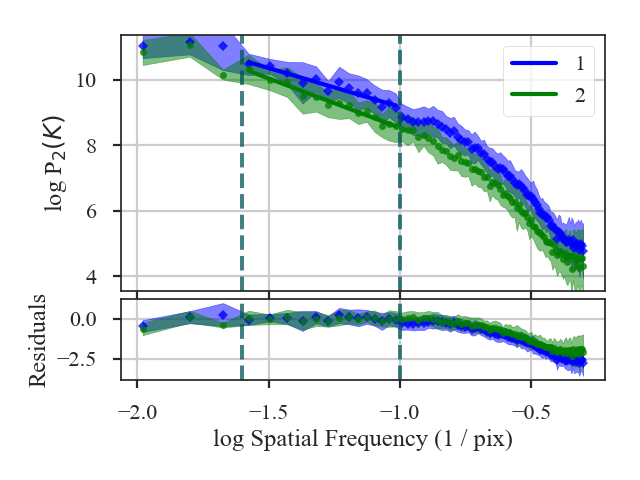
The fit summaries and a plot of the power-spectra with their fits are returned when verbose=True. Colours, labels, and symbols can be altered in the plot with the keywords plot_kwargs1 and plot_kwargs2 in distance_metric.
- The distance between these two images is:
>>> pspec.distance  # doctest: +SKIP
3.0952798493530262
Recomputing an already compute power-spectrum can be avoided by passing a pre-computed PowerSpectrum instead of a dataset. See the distance metric introduction.