SCF Distance
See the tutorial for a description of the Spectral Correlation Function (SCF).
The SCF creates a surface by shifting a spectral-line cube and calculating the correlation of the shifted cube with the original cube. The distance metric defined in SCF_Distance is the L2 distance between the correlation surfaces, weighted by the inverse of the lag:
where \(S_i\) is the correlation surface and \(\ell\) is the spatial lag between the shifted and original cubes.
This direct comparison between the correlation surfaces requires that a common set of spatial lags be used. SCF_Distance creates a common set of angular lags to compare two data cubes.
More information on the distance metric definitions can be found in Koch et al. 2017
Using
The data in this tutorial are available here.
We need to import the SCF_Distance class, along with a few other common packages:
>>> from turbustat.statistics import SCF_Distance
>>> from astropy.io import fits
>>> import matplotlib.pyplot as plt
SCF_Distance takes two data cubes as input:
>>> cube = fits.open("Design4_flatrho_0021_00_radmc.fits")[0]  # doctest: +SKIP
>>> cube_fid = fits.open("Fiducial0_flatrho_0021_00_radmc.fits")[0]  # doctest: +SKIP
>>> scf = SCF_Distance(cube_fid, cube, size=11)  # doctest: +SKIP
This call runs SCF for the two cubes, which can be accessed with scf1 and scf2.
The default setting assumes that the boundaries are continuous (e.g., simulated observations from a periodic-box simulation, like this example). To change how boundaries are handled, boundary can be set in SCF_Distance. For example, for observational data, boundary='cut' should be used. When comparing a simulated observation to a real observation, different boundary conditions can be given: boundary=['cut', 'continuous']. The first list item will be used for the first cube given to SCF_Distance and the same for the second list item.
To calculate the distance between the cubes:
>>> scf.distance_metric(verbose=True) # doctest: +SKIP
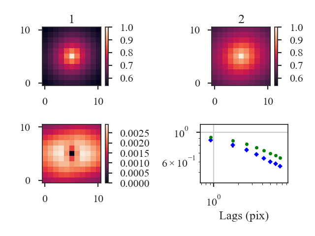
With verbose=True, this function creates a plot of the SCF correlation surfaces (top row), the weighted difference between the surfaces (left, second row), and azimuthally-averaged SCF curves for both cubes (right, second row).
The distance between the SCF surfaces is:
>>> scf.distance  # doctest: +SKIP
0.08101015924738914
By default, the distance between the surfaces is weighted by the lag (see equation above). This weighting can be disabled by setting weighted=False in distance_metric, and the distance metrics reduces to the L2 norm between the surfaces.
A pre-computed SCF class can be also passed instead of a data cube. However, the SCF will need to be recomputed if the lags are different from the common set defined in SCF_Distance. See the distance metric introduction.