VCA Distance
See the tutorial for a description of Velocity Channel Analysis (VCA).
The VCA distance is defined as the t-statistic of the difference in the fitted slopes:
\(\beta_i\) are the slopes of the VCA spectra and \(\sigma_{\beta_i}\) are the uncertainty of the slopes.
More information on the distance metric definitions can be found in Koch et al. 2017.
Using
The data in this tutorial are available here.
We need to import the VCA_Distance class, along with a few other common packages:
>>> from turbustat.statistics import VCA_Distance
>>> from astropy.io import fits
>>> import matplotlib.pyplot as plt
>>> import astropy.units as u
VCA_Distance takes two data cubes as input:
>>> cube = fits.open("Design4_flatrho_0021_00_radmc.fits")[0]  # doctest: +SKIP
>>> cube_fid = fits.open("Fiducial0_flatrho_0021_00_radmc.fits")[0]  # doctest: +SKIP
From the VCA tutorial, we know that limits should be placed on the power-spectra. These limits can be specified with low_cut and high_cut:
>>> vca = VCA_Distance(cube_fid, cube, low_cut=0.025 / u.pix,
...                    high_cut=0.1 / u.pix)  # doctest: +SKIP
This will run VCA on the given cubes, which can be accessed as vca1 and vca2.
Additional parameters can be specified to VCA. Different fit limits for the two cubes can be given as a two-element list (e.g., low_cut=[0.025 / u.pix, 0.04 / u.pix]). Estimated break points in the power-spectra can be given in the same format, which will enable fitting with a broken-linear model.
- To find the distance between the cubes:
>>> vca.distance_metric(verbose=True)  # doctest: +SKIP
                            OLS Regression Results
==============================================================================
Dep. Variable:                      y   R-squared:                       0.985
Model:                            OLS   Adj. R-squared:                  0.984
Method:                 Least Squares   F-statistic:                     436.3
Date:                Fri, 16 Nov 2018   Prob (F-statistic):           8.40e-11
Time:                        10:16:28   Log-Likelihood:                 22.506
No. Observations:                  14   AIC:                            -41.01
Df Residuals:                      12   BIC:                            -39.73
Df Model:                           1
Covariance Type:                  HC3
==============================================================================
                 coef    std err          z      P>|z|      [0.025      0.975]
------------------------------------------------------------------------------
const          5.0853      0.137     37.170      0.000       4.817       5.353
x1            -2.3350      0.112    -20.887      0.000      -2.554      -2.116
==============================================================================
Omnibus:                        0.981   Durbin-Watson:                   1.483
Prob(Omnibus):                  0.612   Jarque-Bera (JB):                0.712
Skew:                          -0.138   Prob(JB):                        0.700
Kurtosis:                       1.930   Cond. No.                         15.2
==============================================================================
                            OLS Regression Results
==============================================================================
Dep. Variable:                      y   R-squared:                       0.986
Model:                            OLS   Adj. R-squared:                  0.985
Method:                 Least Squares   F-statistic:                     722.3
Date:                Fri, 16 Nov 2018   Prob (F-statistic):           4.33e-12
Time:                        10:16:28   Log-Likelihood:                 18.704
No. Observations:                  14   AIC:                            -33.41
Df Residuals:                      12   BIC:                            -32.13
Df Model:                           1
Covariance Type:                  HC3
==============================================================================
                 coef    std err          z      P>|z|      [0.025      0.975]
------------------------------------------------------------------------------
const          3.6086      0.141     25.636      0.000       3.333       3.884
x1            -3.2136      0.120    -26.876      0.000      -3.448      -2.979
==============================================================================
Omnibus:                       13.847   Durbin-Watson:                   2.394
Prob(Omnibus):                  0.001   Jarque-Bera (JB):                9.666
Skew:                          -1.631   Prob(JB):                      0.00796
Kurtosis:                       5.434   Cond. No.                         15.2
==============================================================================
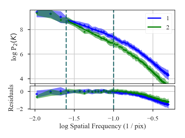
This function returns a summary of the fits to the VCA spectra and plots the two spectra with the fits. Colours, symbols and labels in the plot can be changed with plot_kwargs1 and plot_kwargs2 in distance_metric.
- The distance is:
>>> vca.distance  # doctest: +SKIP
5.366955632554179
Changing the width of the velocity channels affects the contribution of the turbulent velocity field to the spectrum, thereby altering the measured index (Lazarian & Pogosyan 2000). It is generally advisable to compare cubes with a similar velocity resolution.
In VCA_Distance, the channel width can be changed with channel_width. The new channel width should be (1) larger than the current channel widths of the cubes, and (2) in similar units to the spectral axis of the cubes (i.e., a width in velocity should be given for a spectral axis in velocity).
Warning
Changing the spectral resolution will be slow for large cubes. Consider changing the velocity resolution of large cubes before running VCA.
In this example, we will change the velocity resolution to 400 m/s:
>>> vca = VCA_Distance(cube_fid, cube, low_cut=0.025 / u.pix,
...                    high_cut=0.1 / u.pix, channel_width=400 * u.m / u.s)  # doctest: +SKIP
>>> vca.distance_metric(verbose=True)  # doctest: +SKIP
                            OLS Regression Results
==============================================================================
Dep. Variable:                      y   R-squared:                       0.985
Model:                            OLS   Adj. R-squared:                  0.983
Method:                 Least Squares   F-statistic:                     419.3
Date:                Fri, 16 Nov 2018   Prob (F-statistic):           1.06e-10
Time:                        10:16:28   Log-Likelihood:                 22.121
No. Observations:                  14   AIC:                            -40.24
Df Residuals:                      12   BIC:                            -38.96
Df Model:                           1
Covariance Type:                  HC3
==============================================================================
                 coef    std err          z      P>|z|      [0.025      0.975]
------------------------------------------------------------------------------
const          3.0105      0.141     21.350      0.000       2.734       3.287
x1            -2.3639      0.115    -20.478      0.000      -2.590      -2.138
==============================================================================
Omnibus:                        0.854   Durbin-Watson:                   1.515
Prob(Omnibus):                  0.652   Jarque-Bera (JB):                0.676
Skew:                          -0.144   Prob(JB):                        0.713
Kurtosis:                       1.963   Cond. No.                         15.2
==============================================================================
                            OLS Regression Results
==============================================================================
Dep. Variable:                      y   R-squared:                       0.985
Model:                            OLS   Adj. R-squared:                  0.984
Method:                 Least Squares   F-statistic:                     684.5
Date:                Fri, 16 Nov 2018   Prob (F-statistic):           5.94e-12
Time:                        10:16:28   Log-Likelihood:                 17.855
No. Observations:                  14   AIC:                            -31.71
Df Residuals:                      12   BIC:                            -30.43
Df Model:                           1
Covariance Type:                  HC3
==============================================================================
                 coef    std err          z      P>|z|      [0.025      0.975]
------------------------------------------------------------------------------
const          1.5197      0.146     10.408      0.000       1.234       1.806
x1            -3.2379      0.124    -26.163      0.000      -3.481      -2.995
==============================================================================
Omnibus:                       13.778   Durbin-Watson:                   2.379
Prob(Omnibus):                  0.001   Jarque-Bera (JB):                9.575
Skew:                          -1.633   Prob(JB):                      0.00833
Kurtosis:                       5.398   Cond. No.                         15.2
==============================================================================
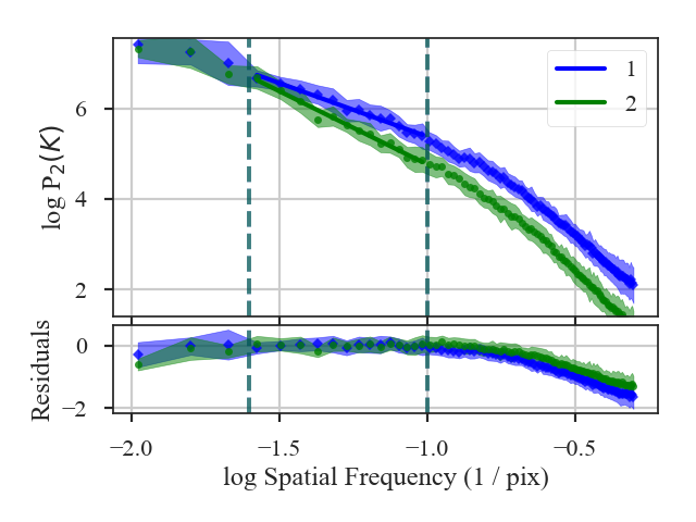
The VCA power-spectra with 400 m/s channels have a similar slope to the original velocity resolution. The distance then has not significantly changed:
>>> vca.distance  # doctest: +SKIP
5.164776059129051
A pre-computed VCA class can be also passed instead of a data cube. See the distance metric introduction.