VCS Distance
See the tutorial for a description of Velocity Coordinate Spectrum (VCS).
There are two asymptotic regimes of the VCS corresponding to high and low resolution (Lazarian & Pogosyan 2006). The transition between these regimes depends on the spatial resolution (i.e., beam size) of the data, the spectral resolution of the data, and the velocity dispersion. The current VCS implementation in TurbuStat fits a broken linear model to approximate the asymptotic regimes, rather than fitting with the full VCS formalism (Chepurnov et al. 2010, Chepurnov et al. 2015). We assume that the break point lies at the transition point between the regimes and label velocity frequencies smaller than the break as “large-scale” and frequencies larger than the break as “small-scale”.
There are four distance definitions for the VCS based on the broken linear modelling described above. All of these distance metrics are based on t-statistics between the VCS for each cube:
- The difference between the fitted slopes on “large-scales” (below the break position):
large_scale_distance. - \[d_{\rm large-scale} = \frac{|\beta_{{\rm LS}, 1} - \beta_{{\rm LS}, 2}|}{\sqrt{\sigma_{\beta_{{\rm LS}, 1}}^2 + \sigma_{\beta_{{\rm LS}, 2}}^2}}\]
\(\beta_{{\rm LS}, i}\) are the slopes of the VCS on large-scales and \(\sigma_{\beta_{{\rm LS}, i}}\) are the uncertainty of the slopes.
- The difference between the fitted slopes on “large-scales” (below the break position):
- The difference between the fitted slopes on “small-scales” (above the break position):
small_scale_distance. - \[d_{\rm small-scale} = \frac{|\beta_{{\rm SS}, 1} - \beta_{{\rm SS}, 2}|}{\sqrt{\sigma_{\beta_{{\rm SS}, 1}}^2 + \sigma_{\beta_{{\rm SS}, 2}}^2}}\]
\(\beta_{{\rm SS}, i}\) are the slopes of the VCS on small-scales and \(\sigma_{\beta_{{\rm SS}, i}}\) are the uncertainty of the slopes.
- The difference between the fitted slopes on “small-scales” (above the break position):
- The sum of the differences between the slopes in both regimes:
distance - \[d_{{\rm all}} = d_{\rm large-scale} + d_{\rm small-scale}\]
- The sum of the differences between the slopes in both regimes:
- The difference in the fitted break points:
break_distance - \[d_{\rm break} = \frac{|b_{1} - b_{2}|}{\sqrt{\sigma_{b_{1}}^2 + \sigma_{b_{2}}^2}}\]
\(b_{i}\) are the break locations of the VCS and \(\sigma_{b_{i}}\) are the uncertainties.
- The difference in the fitted break points:
More information on the distance metric definitions can be found in Koch et al. 2017.
Using
The data in this tutorial are available here.
We need to import the VCS_Distance class, along with a few other common packages:
>>> from turbustat.statistics import VCS_Distance
>>> from astropy.io import fits
>>> import matplotlib.pyplot as plt
>>> import astropy.units as u
VCS_Distance takes two data cubes as input:
>>> cube = fits.open("Design4_flatrho_0021_00_radmc.fits")[0]  # doctest: +SKIP
>>> cube_fid = fits.open("Fiducial0_flatrho_0021_00_radmc.fits")[0]  # doctest: +SKIP
From the VCS tutorial, we know that limits should be placed on the power-spectra. These limits can be specified with low_cut and high_cut:
>>> vcs = VCS_Distance(cube_fid, cube,
...                    fit_kwargs=dict(low_cut=0.025 / u.pix,
...                                    high_cut=0.1 / u.pix))  # doctest: +SKIP
This will run VCS on the given cubes, which can be accessed as vcs1 and vcs2.
Settings for the VCS fitting can be passed with fit_kwargs, and fit_kwargs2 when different setting are required for the second cube. In this example, we set the fitting limits to be used.
- To find the distances between the cube:
>>> vcs.distance_metric(verbose=True)  # doctest: +SKIP
                            OLS Regression Results
==============================================================================
Dep. Variable:                      y   R-squared:                       0.993
Model:                            OLS   Adj. R-squared:                  0.992
Method:                 Least Squares   F-statistic:                     3678.
Date:                Fri, 16 Nov 2018   Prob (F-statistic):           1.96e-86
Time:                        11:20:09   Log-Likelihood:                -17.089
No. Observations:                  85   AIC:                             42.18
Df Residuals:                      81   BIC:                             51.95
Df Model:                           3
Covariance Type:            nonrobust
==============================================================================
                 coef    std err          t      P>|t|      [0.025      0.975]
------------------------------------------------------------------------------
const          1.2848      0.295      4.354      0.000       0.698       1.872
x1            -2.1220      0.171    -12.428      0.000      -2.462      -1.782
x2           -14.5354      0.317    -45.812      0.000     -15.167     -13.904
x3             0.0715      0.129      0.553      0.582      -0.186       0.329
==============================================================================
Omnibus:                        2.570   Durbin-Watson:                   0.089
Prob(Omnibus):                  0.277   Jarque-Bera (JB):                2.546
Skew:                          -0.378   Prob(JB):                        0.280
Kurtosis:                       2.616   Cond. No.                         21.5
==============================================================================
                            OLS Regression Results
==============================================================================
Dep. Variable:                      y   R-squared:                       0.988
Model:                            OLS   Adj. R-squared:                  0.987
Method:                 Least Squares   F-statistic:                     2212.
Date:                Fri, 16 Nov 2018   Prob (F-statistic):           1.43e-77
Time:                        11:20:09   Log-Likelihood:                -38.551
No. Observations:                  85   AIC:                             85.10
Df Residuals:                      81   BIC:                             94.87
Df Model:                           3
Covariance Type:            nonrobust
==============================================================================
                 coef    std err          t      P>|t|      [0.025      0.975]
------------------------------------------------------------------------------
const          1.5246      0.380      4.014      0.000       0.769       2.280
x1            -1.9578      0.220     -8.908      0.000      -2.395      -1.520
x2           -14.7109      0.408    -36.020      0.000     -15.524     -13.898
x3             0.1178      0.167      0.707      0.482      -0.214       0.449
==============================================================================
Omnibus:                        7.714   Durbin-Watson:                   0.059
Prob(Omnibus):                  0.021   Jarque-Bera (JB):                3.123
Skew:                          -0.127   Prob(JB):                        0.210
Kurtosis:                       2.096   Cond. No.                         21.5
==============================================================================
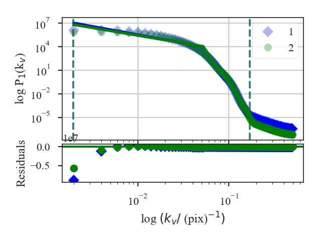
This function returns a summary of the broken linear fits to the VCS for each cube. The plot shows the VCS for both cubes; in this example, the two are quite similar.
The distances between the cubes, as defined above, are:
>>> vcs.large_scale_distance  # doctest: +SKIP
0.5901343561262037
>>> vcs.small_scale_distance  # doctest: +SKIP
0.01921401163828633
>>> vcs.distance  # doctest: +SKIP
0.60934836776449
>>> vcs.break_distance  # doctest: +SKIP
0.0023172070537929865
The difference in the slopes is dominated by vcs.large_scale_distance, while the small-scale slopes are quite similar. The break locations are also similar and give a small vcs.break_distance.
A pre-computed VCS class can be also passed instead of a data cube. See the distance metric introduction.