Creating testing data
TurbuStat includes a simulation package to create 2D images and PPV cubes with set power-law indices. These provide simple non-realistic synthetic observations that can be used to test idealized regimes of turbulent statistics.:
>>> import matplotlib.pyplot as plt
>>> from astropy.io import fits
Two-dimensional images
- The 2D power-law image function is
make_extended:: >>> from turbustat.simulator import make_extended
The make_extended function is adapted from the implementation in image_registration.
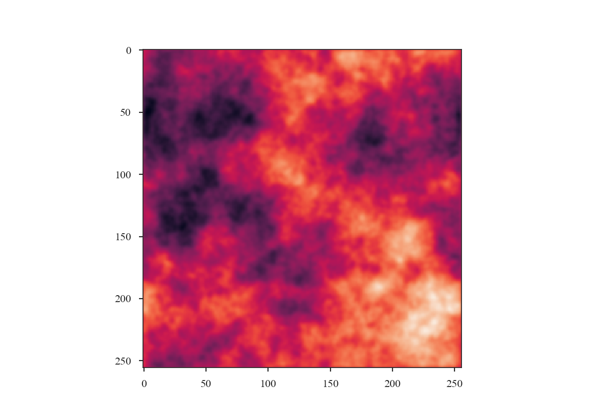
To create an isotropic power-law field, or a fractional Brownian Motion (fBM) field, with an index of 3 and size of 256 pixels, we run:
>>> rnoise_img = make_extended(256, powerlaw=3.)
>>> plt.imshow(rnoise_img)
To calculate the power-spectrum and check its index, we need to generate a minimal FITS HDU:
>>> rnoise_hdu = fits.PrimaryHDU(rnoise_img)
The FITS header lacks the information to convert to angular or physical scales and is used here to show the minimal working case. See the handling simulated data tutorial on how to create usable FITS header for simulated data.
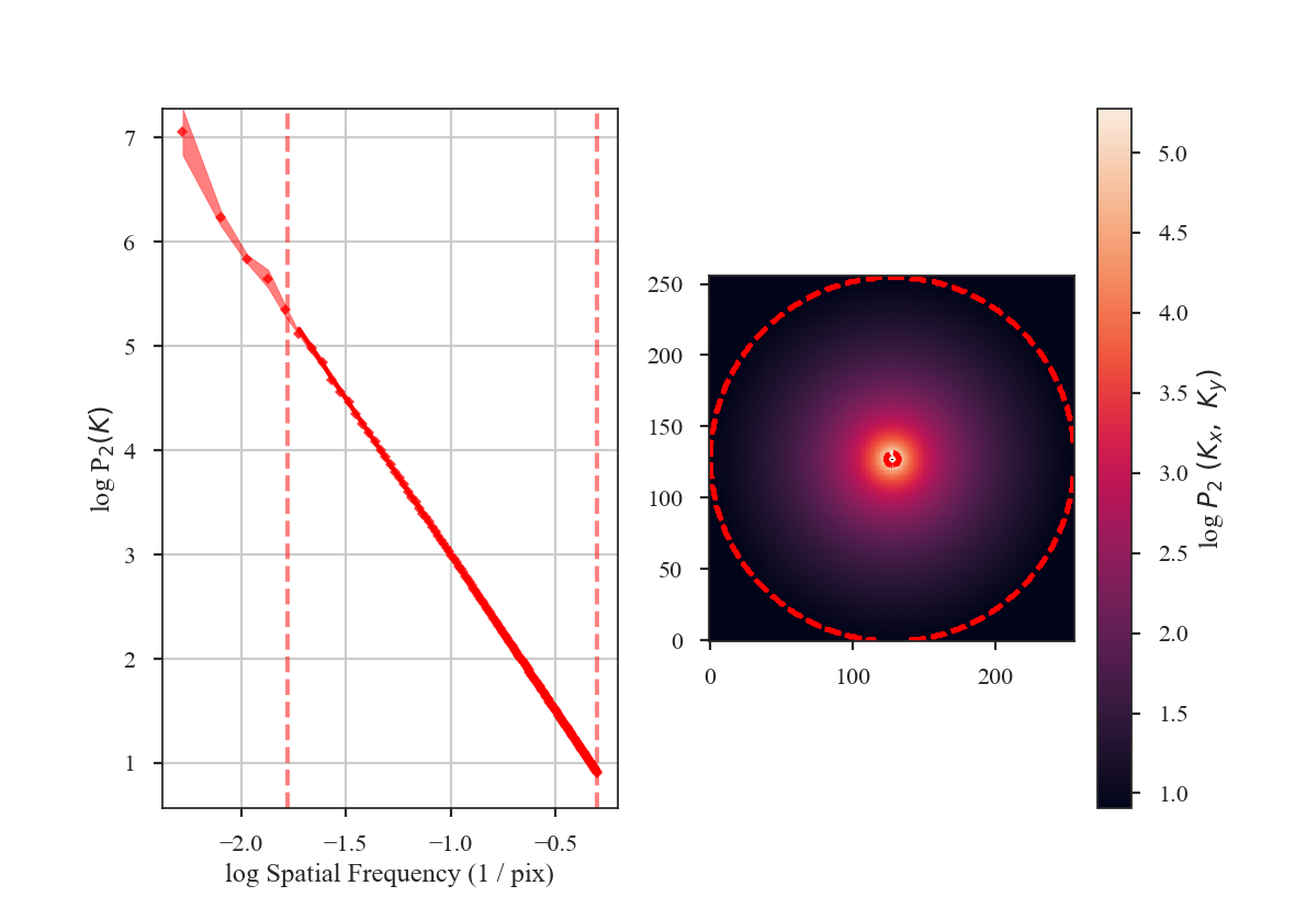
The power-spectrum of the image should give a slope of 3:
>>> from turbustat.statistics import PowerSpectrum
>>> pspec = PowerSpectrum(rnoise_hdu)
>>> pspec.run(verbose=True, radial_pspec_kwargs={'binsize': 1.0},
...           fit_kwargs={'weighted_fit': True}, fit_2D=False,
...           low_cut=1. / (60 * u.pix))
                            OLS Regression Results
==============================================================================
Dep. Variable:                      y   R-squared:                       1.000
Model:                            OLS   Adj. R-squared:                  1.000
Method:                 Least Squares   F-statistic:                 8.070e+06
Date:                Thu, 21 Jun 2018   Prob (F-statistic):               0.00
Time:                        11:43:47   Log-Likelihood:                 701.40
No. Observations:                 177   AIC:                            -1399.
Df Residuals:                     175   BIC:                            -1392.
Df Model:                           1
Covariance Type:            nonrobust
==============================================================================
                 coef    std err          t      P>|t|      [0.025      0.975]
------------------------------------------------------------------------------
const          0.0032      0.001      3.952      0.000       0.002       0.005
x1            -2.9946      0.001  -2840.850      0.000      -2.997      -2.992
==============================================================================
Omnibus:                      252.943   Durbin-Watson:                   1.077
Prob(Omnibus):                  0.000   Jarque-Bera (JB):            26797.433
Skew:                          -5.963   Prob(JB):                         0.00
Kurtosis:                      62.087   Cond. No.                         4.55
==============================================================================
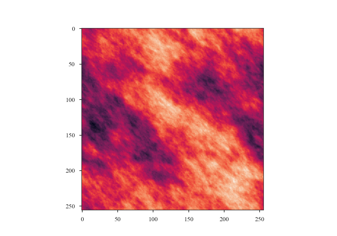
Anisotropic 2D images can also be produced:
>>> import astropy.units as u
>>> rnoise_img = make_extended(256, powerlaw=3., ellip=0.5, theta=45 * u.deg)
>>> plt.imshow(rnoise_img)
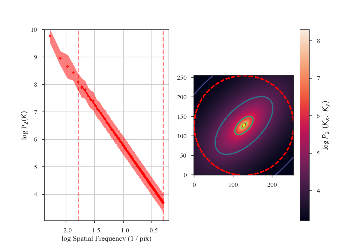
The power-spectrum can then be calculated and fit in 1D and 2D (see Spatial Power Spectrum):
>>> pspec = PowerSpectrum(rnoise_hdu)
>>> pspec.run(verbose=True, radial_pspec_kwargs={'binsize': 1.0},
...           fit_kwargs={'weighted_fit': True}, fit_2D=False,
...           low_cut=1. / (60 * u.pix))
                            OLS Regression Results
==============================================================================
Dep. Variable:                      y   R-squared:                       1.000
Model:                            OLS   Adj. R-squared:                  1.000
Method:                 Least Squares   F-statistic:                 1.122e+06
Date:                Wed, 15 Aug 2018   Prob (F-statistic):               0.00
Time:                        14:18:14   Log-Likelihood:                 526.68
No. Observations:                 177   AIC:                            -1049.
Df Residuals:                     175   BIC:                            -1043.
Df Model:                           1
Covariance Type:            nonrobust
==============================================================================
                 coef    std err          t      P>|t|      [0.025      0.975]
------------------------------------------------------------------------------
const          2.7786      0.002   1295.906      0.000       2.774       2.783
x1            -2.9958      0.003  -1059.077      0.000      -3.001      -2.990
==============================================================================
Omnibus:                       35.156   Durbin-Watson:                   2.661
Prob(Omnibus):                  0.000   Jarque-Bera (JB):              334.753
Skew:                           0.205   Prob(JB):                     2.04e-73
Kurtosis:                       9.725   Cond. No.                         4.55
==============================================================================
Three-dimensional fields
Three-dimensional power-law fields can also be produced with make_3dfield:
>>> from turbustat.simulator import make_3dfield
>>> threeD_field = make_3dfield(128, powerlaw=3.)
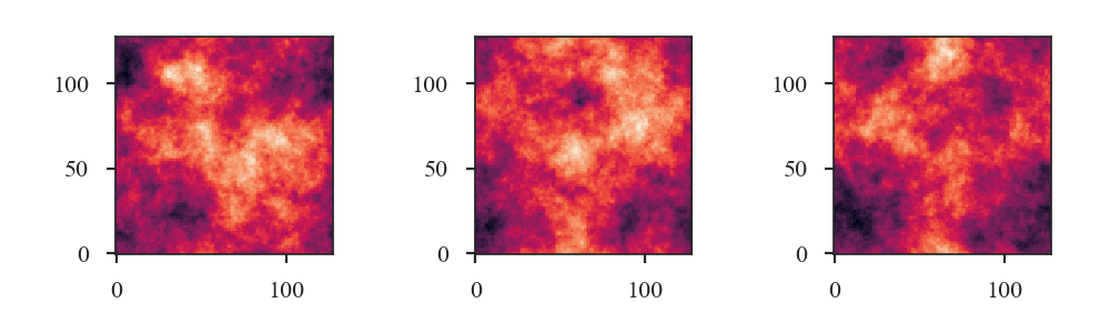
Only isotropic fields can currently be created. Projections of this 3D field are shown below:
>>> plt.figure(figsize=[10, 3])
>>> plt.subplot(131)
>>> plt.imshow(threeD_field.mean(0), origin='lower')
>>> plt.subplot(132)
>>> plt.imshow(threeD_field.mean(1), origin='lower')
>>> plt.subplot(133)
>>> plt.imshow(threeD_field.mean(2), origin='lower')
>>> plt.tight_layout()
Simple PPV cubes
Also included in this module is a simple PPV cube generator. It has many restrictions and is primarily intended for creating idealized optically-thin 21-cm HI emission to test turbulent statistics in idealized conditions.
The function to create the cubes is:
>>> from turbustat.simulator import make_3dfield, make_ppv
>>> import astropy.units as u
We need to create 3D velocity and density cubes. For this simple example, we will create small 32 pixel cubes so this is quick to compute:
>>> velocity = make_3dfield(32, powerlaw=4., amp=1.,
...                         randomseed=98734) * u.km / u.s
>>> density = make_3dfield(32, powerlaw=3., amp=1.,
...                        randomseed=328764) * u.cm**-3
Both fields need to have appropriate units.
There is an additional issue for the density field generated from a power-law in that it will contain negative values. There are numerous approaches to account for negative values, including adding the minimum to force all values to be positive or taking the exponential of this field to produce a log-normal field (Brunt & Heyer 2002, Roman-Duval et al. 2011). Here we use the approach from Ossenkopf et al. 2006, adding one standard deviation to all values and masking values that remain negative. Each of these approaches will distort the field properties to some extent.
>>> density += density.std()
>>> density[density.value < 0.] = 0. * u.cm**-3
To produce a PPV cube from these fields, using the zeroth axis as the line-of-sight:
>>> cube_hdu = make_ppv(velocity, density, los_axis=0,
...                     T=100 * u.K, chan_width=0.5 * u.km / u.s,
...                     v_min=-20 * u.km / u.s,
...                     v_max=20 * u.km / u.s)
We will demonstrate the cube properties using spectral-cube:
>>> from spectral_cube import SpectralCube
>>> cube = SpectralCube.read(cube_hdu)
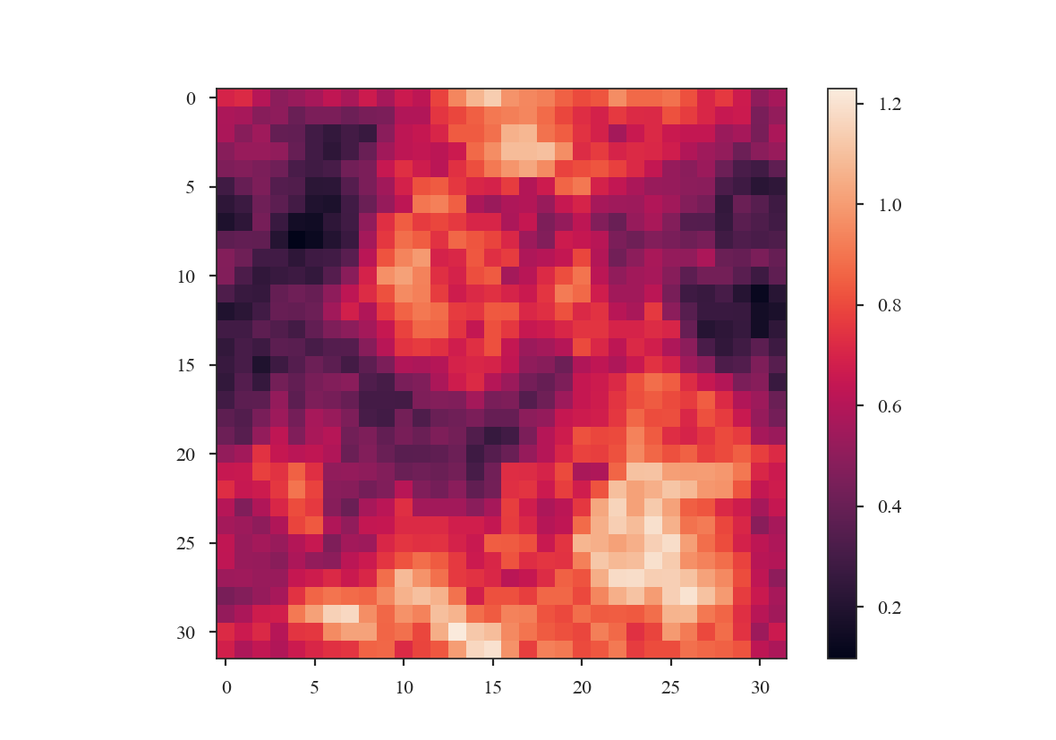
The zeroth moment, integrated over the velocity axis:
>>> cube.moment0().quicklook()
>>> plt.colorbar()
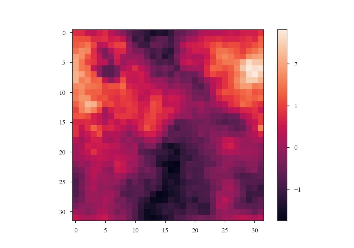
The velocity centroid map:
>>> cube.moment1().quicklook()
>>> plt.colorbar()
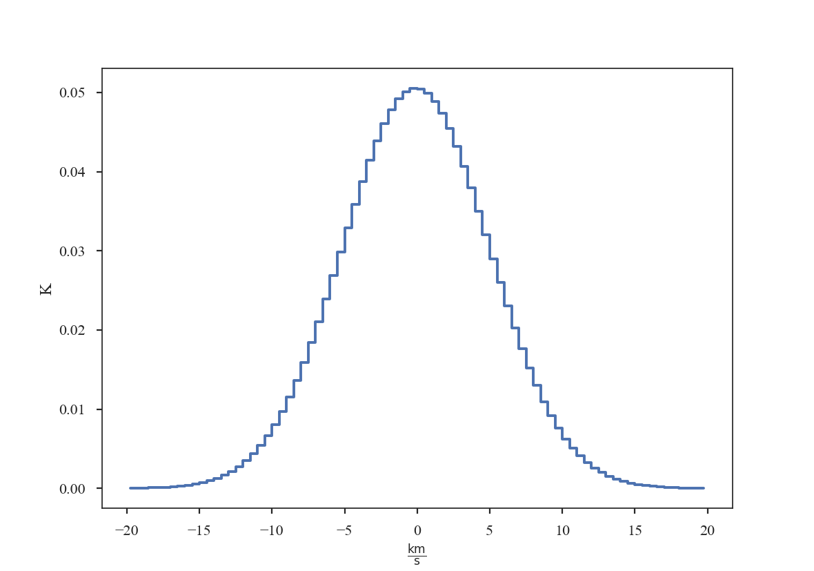
And the mean spectrum, averaged over the spatial dimensions:
>>> cube.mean(axis=(1, 2)).quicklook()
Warning
These simulated cubes (and those from other numerical methods) will suffer from “shot noise” due to a finite number of emitting sources along the line of sight. This will lead to deviations of expected behaviours for several statistics, most notably the VCA and VCS methods. See Esquivel et al. 2003 and Chepurnov et al. 2009 for thorough explanations of this effect.
Useful references for making mock-HI cubes include:
Source Code
Functions
|
Generate a 3D power-law field with a specified index and random phases. |
|
Generate a 2D power-law image with a specified index and random phases. |
|
Generate a mock, optically-thin HI PPV cube from a given velocity and density field. |