Spatial Power Spectrum
Overview
A common analysis technique for two-dimensional images is the spatial power spectrum – the square of the 2D Fourier transform of an image. A radial profile of the 2D power spectrum gives the 1D power spectrum. The slope of this 1D spectrum can be compared to the expected indices in different physical limits. For example, the velocity field of Kolmogorov turbulence follows \(k^{-5/3}\), while Burgers’ turbulence has \(k^{-2}\).
However, observations are a combination of both velocity and density fluctuations (e.g., Lazarian & Pogosyan 2000), and the measured index from an integrated intensity map depend on both components, as well as optical depth effects. For a turbulent optically thin tracer, an integrated intensity image (or zeroth moment) will have \(k^{-11/3}\), while an optically thick tracer saturates to \(k^{-3}\) (Lazarian & Pogosyan 2004, Burkhart et al. 2013). The effect of velocity resolution is discussed in the VCA tutorial.
Using
The data in this tutorial are available here.
We need to import the PowerSpectrum code, along with a few other common packages:
>>> from turbustat.statistics import PowerSpectrum
>>> from astropy.io import fits
And we load in the data:
>>> moment0 = fits.open("Design4_flatrho_0021_00_radmc_moment0.fits")[0]
The power spectrum is computed using:
>>> pspec = PowerSpectrum(moment0, distance=250 * u.pc)
>>> pspec.run(verbose=True, xunit=u.pix**-1)
                            OLS Regression Results
==============================================================================
Dep. Variable:                      y   R-squared:                       0.941
Model:                            OLS   Adj. R-squared:                  0.941
Method:                 Least Squares   F-statistic:                     1426.
Date:                Fri, 29 Sep 2017   Prob (F-statistic):           1.44e-56
Time:                        14:32:47   Log-Likelihood:                -52.829
No. Observations:                  91   AIC:                             109.7
Df Residuals:                      89   BIC:                             114.7
Df Model:                           1
Covariance Type:            nonrobust
==============================================================================
                 coef    std err          t      P>|t|      [0.025      0.975]
------------------------------------------------------------------------------
const          3.1677      0.103     30.828      0.000       2.964       3.372
x1            -5.0144      0.133    -37.761      0.000      -5.278      -4.751
==============================================================================
Omnibus:                        3.532   Durbin-Watson:                   0.129
Prob(Omnibus):                  0.171   Jarque-Bera (JB):                3.481
Skew:                          -0.468   Prob(JB):                        0.175
Kurtosis:                       2.797   Cond. No.                         4.40
==============================================================================
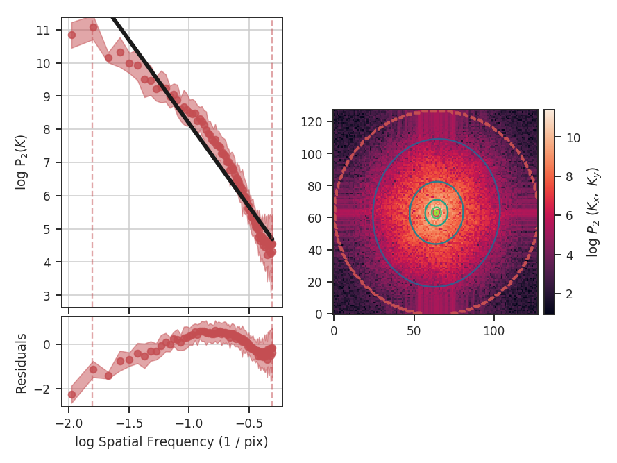
The code returns a summary of the one-dimensional fit and a figure showing the one-dimensional spectrum and model on the left, and the two-dimensional power-spectrum on the right. If fit_2D=True is set in run (the default setting), the contours on the two-dimensional power-spectrum are fit using an elliptical power-law model. The dashed red lines (or contours) on both plots are the limits of the data used in the fits. We use an elliptical power-law model:
Here, the power-law index is \(\Gamma\), the orientation angle of the ellipse with respect to the \(x,y\) coordinate system is given by \(\theta\) and the ellipticity is \(q\in [0,1)\).
The power spectrum of this simulation has a slope of \(-3.3\pm0.1\), but the power-spectrum deviates from a single power-law on small scales. This is due to the the limited inertial range in this simulation. The spatial frequencies used in the fit can be limited by setting low_cut and high_cut. The inputs should have frequency units in pixels, angle, or physical units. For example,
>>> pspec.run(verbose=True, xunit=u.pix**-1, low_cut=0.025 / u.pix,
...           high_cut=0.1 / u.pix)
                            OLS Regression Results
==============================================================================
Dep. Variable:                      y   R-squared:                       0.971
Model:                            OLS   Adj. R-squared:                  0.968
Method:                 Least Squares   F-statistic:                     398.6
Date:                Thu, 28 Sep 2017   Prob (F-statistic):           1.42e-10
Time:                        17:02:20   Log-Likelihood:                 14.077
No. Observations:                  14   AIC:                            -24.15
Df Residuals:                      12   BIC:                            -22.87
Df Model:                           1
Covariance Type:            nonrobust
==============================================================================
                 coef    std err          t      P>|t|      [0.025      0.975]
------------------------------------------------------------------------------
const          5.5109      0.190     29.021      0.000       5.097       5.925
x1            -3.0223      0.151    -19.964      0.000      -3.352      -2.692
==============================================================================
Omnibus:                        0.901   Durbin-Watson:                   2.407
Prob(Omnibus):                  0.637   Jarque-Bera (JB):                0.718
Skew:                          -0.215   Prob(JB):                        0.698
Kurtosis:                       1.977   Cond. No.                         15.2
==============================================================================

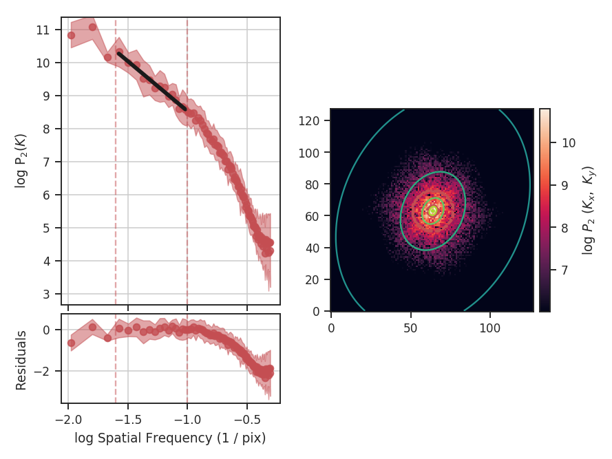
When limiting the fit to the inertial range, the slope is \(-3.0\pm0.2\). low_cut and high_cut can also be given as spatial frequencies in angular units (e.g., u.deg**-1). And since a distance was specified, the low_cut and high_cut can also be given in physical frequency units (e.g., u.pc**-1).
The fit to the two-dimensional power-spectrum has also changed. These parameters aren’t included in the fit summary for the 1D fit. Instead, they can be accessed through:
>>> print(pspec.slope2D, pspec.slope2D_err)
(-3.155235947194412, 0.19744198375014044)
>>> print(pspec.ellip2D, pspec.ellip2D_err)
(0.74395734515060385, 0.043557506230624203)
>>> print(pspec.theta2D, pspec.theta2D_err)
(1.1364954648370515, 0.09436799399259721)
The slope is moderately steeper than in the 1D model, but within the respective uncertainty ranges. By default, the parameter uncertainties for the 2D model are determined by a bootstrap. After fitting the model, the residuals are resampled and added back to the data. The resampled data are then fit to the model. This procedure is repeated some number of times (the default is 100) to build up distributions for the fit parameters. The bootstrap estimation is enabled in the code by setting the bootstrap keyword to True in fit_2Dpspec and the number of iterations is set with niters (the default is 100). These can be set in run by passing a keyword dictionary to fit_2D_kwargs (e.g., fit_2D_kwargs={'bootstrap': False}). The other parameters are the ellipticity, which is bounded between 0 and 1 (with 1 being circular), and theta, the angle between the x-axis and the semi-major axis of the ellipse. Theta is bounded between 0 and \(\pi\). The 2D power spectrum here is moderately anisotropic.
Breaks in the power-law behaviour in observations (and higher-resolution simulations) can result from differences in the physical processes dominating at those scales (e.g., Swift & Welch 2008). To capture this behaviour, PowerSpectrum can be passed a break point to enable fitting with a segmented linear model (Lm_Seg):
>>> pspec = PowerSpectrum(moment0, distance=250 * u.pc)
>>> pspec.run(verbose=True, xunit=u.pc**-1, low_cut=0.02 / u.pix, high_cut=0.4 / u.pix,
...           fit_kwargs={'brk': 0.1 / u.pix, 'log_break': False}, fit_2D=False)
                            OLS Regression Results
==============================================================================
Dep. Variable:                      y   R-squared:                       0.996
Model:                            OLS   Adj. R-squared:                  0.995
Method:                 Least Squares   F-statistic:                     4904.
Date:                Fri, 29 Sep 2017   Prob (F-statistic):           1.84e-77
Time:                        14:29:10   Log-Likelihood:                 61.421
No. Observations:                  70   AIC:                            -114.8
Df Residuals:                      66   BIC:                            -105.8
Df Model:                           3
Covariance Type:            nonrobust
==============================================================================
                 coef    std err          t      P>|t|      [0.025      0.975]
------------------------------------------------------------------------------
const          5.1169      0.087     59.057      0.000       4.944       5.290
x1            -3.3384      0.082    -40.924      0.000      -3.501      -3.176
x2            -4.9624      0.191    -26.043      0.000      -5.343      -4.582
x3            -0.0084      0.048     -0.174      0.863      -0.105       0.088
==============================================================================
Omnibus:                        3.812   Durbin-Watson:                   1.096
Prob(Omnibus):                  0.149   Jarque-Bera (JB):                2.211
Skew:                          -0.191   Prob(JB):                        0.331
Kurtosis:                       2.218   Cond. No.                         22.4
==============================================================================
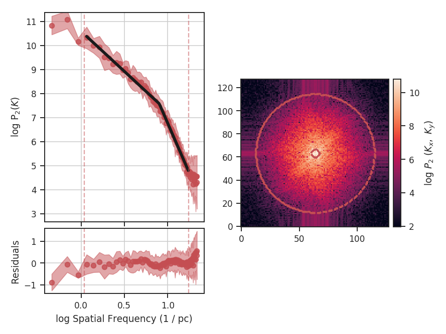
brk is the initial guess for where the break point location is. Here I’ve set it to the extent of the inertial range of the simulation. log_break should be enabled if the given brk is already the log (base-10) value (since the fitting is done in log-space). The segmented linear model iteratively optimizes the location of the break point, trying to minimize the gap between the different components. This is the x3 parameter above. The slopes of the components are x1 and x2, but the second slope is defined relative to the first slope (i.e., if x2=0, the slopes of the components would be the same). The true slopes can be accessed through pspec.slope and pspec.slope_err. The location of the fitted break point is given by pspec.brk, and its uncertainty pspec.brk_err. If the fit does not find a good break point, it will revert to a linear fit without the break.
Note that the 2D fitting was disabled in this last example. The 2D model cannot fit a break point, and will instead try to fit a single power-law for the between low_cut and high_cut, which we know already know is the wrong model. Thus, it has been disabled to avoid confusion. A strategy for fitting the 2D model when the spectrum shows a break is to first fit the 1D model, find the break point, and then fit the 2D spectrum independently using the break point as the high_cut in fit_2Dpspec.
There may be cases where you want to limit the azimuthal angles used to create the 1D averaged power-spectrum. This may be useful if, for example, you want to find a measure of anistropy but the 2D power-law fit is not performing well. We will add extra constraints to the previous example with a break point:
>>> pspec = PowerSpectrum(moment0, distance=250 * u.pc)
>>> pspec.run(verbose=True, xunit=u.pc**-1, low_cut=0.02 / u.pix, high_cut=0.4 / u.pix,
...           fit_2D=False, fit_kwargs={'brk': 0.1 / u.pix, 'log_break': False},
...           radial_pspec_kwargs={"theta_0": 1.13 * u.rad, "delta_theta": 40 * u.deg})
                            OLS Regression Results
==============================================================================
Dep. Variable:                      y   R-squared:                       0.990
Model:                            OLS   Adj. R-squared:                  0.989
Method:                 Least Squares   F-statistic:                     2113.
Date:                Fri, 29 Sep 2017   Prob (F-statistic):           1.76e-65
Time:                        14:29:10   Log-Likelihood:                 30.377
No. Observations:                  70   AIC:                            -52.75
Df Residuals:                      66   BIC:                            -43.76
Df Model:                           3
Covariance Type:            nonrobust
==============================================================================
                 coef    std err          t      P>|t|      [0.025      0.975]
------------------------------------------------------------------------------
const          5.7150      0.173     33.005      0.000       5.369       6.061
x1            -2.9371      0.154    -19.041      0.000      -3.245      -2.629
x2            -4.9096      0.254    -19.313      0.000      -5.417      -4.402
x3             0.0156      0.077      0.202      0.840      -0.138       0.169
==============================================================================
Omnibus:                        3.679   Durbin-Watson:                   1.837
Prob(Omnibus):                  0.159   Jarque-Bera (JB):                1.894
Skew:                          -0.030   Prob(JB):                        0.388
Kurtosis:                       2.196   Cond. No.                         22.9
==============================================================================
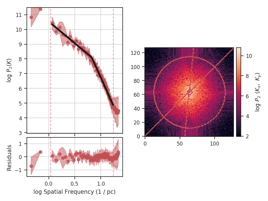
The azimuthal mask has been added onto the plot of the two-dimensional power spectrum. The constraints used here are based on the major axis direction from the two-dimensional fit performed above. This is given as theta_0. The other parameter, delta_theta, is the width of the azimuthal mask to use. Both parameters can be specified in any angular unit.
The default fit uses Ordinary Least Squares. A Weighted Least Squares can be enabled with weighted_fit=True if the segmented linear fit is not used:
>>> pspec = PowerSpectrum(moment0, distance=250 * u.pc)
>>> pspec.run(verbose=True, xunit=u.pix**-1, low_cut=0.025 / u.pix, high_cut=0.1 / u.pix,
...           fit_kwargs={'weighted_fit': True})
                            WLS Regression Results
==============================================================================
Dep. Variable:                      y   R-squared:                       0.969
Model:                            WLS   Adj. R-squared:                  0.966
Method:                 Least Squares   F-statistic:                     372.0
Date:                Fri, 29 Sep 2017   Prob (F-statistic):           2.13e-10
Time:                        15:08:21   Log-Likelihood:                 13.966
No. Observations:                  14   AIC:                            -23.93
Df Residuals:                      12   BIC:                            -22.65
Df Model:                           1
Covariance Type:            nonrobust
==============================================================================
                 coef    std err          t      P>|t|      [0.025      0.975]
------------------------------------------------------------------------------
const          5.5119      0.194     28.476      0.000       5.090       5.934
x1            -3.0200      0.157    -19.288      0.000      -3.361      -2.679
==============================================================================
Omnibus:                        0.701   Durbin-Watson:                   2.387
Prob(Omnibus):                  0.704   Jarque-Bera (JB):                0.655
Skew:                          -0.235   Prob(JB):                        0.721
Kurtosis:                       2.050   Cond. No.                         15.3
==============================================================================
The fit has not changed significantly but may in certain cases.
If strong emission continues to the edge of the map (and the map does not have periodic boundaries), ringing in the FFT can introduce a cross pattern in the 2D power-spectrum. This effect and the use of apodizing kernels to taper the data is covered here.
Most observational data will be smoothed over the beam size, which will steepen the power spectrum on small scales. To account for this, the 2D power spectrum can be divided by the beam response. This is demonstrated here for spatial power-spectra.
References
Many papers have utilized the power spectrum. An incomplete list is provided below: