Velocity Channel Analysis (VCA)
Overview
A major advantage of a spectral-line data cube, rather than an integrated two-dimensional image, is that it captures aspects of both the density and velocity fluctuations in the field of observation. Lazarian & Pogosyan 2000 and Lazarian & Pogosyan 2004 derived how the power spectrum from a cube depends on the statistics of the density and velocity fields for the 21-cm Hydrogen line, allowing for each of their properties to be examined (provided the data have sufficient spectral resolution).
The Lazarian & Pogosyan theory predicts two regimes based on the the power-spectrum slope: the shallow (\(n < -3\)) and the steep (\(n < -3\)) regimes. In the case of optically thick line emission, Lazarian & Pogosyan 2004 show that the slope saturates to \(n = -3\) (see Burkhart et al. 2013 as well). The VCA predictions in these different regimes are shown in Table 1 of Chepurnov & Lazarian 2009 (also see Table 3 in Lazarian 2009). The complementary Velocity Coordinate Spectrum can be used in tandem with VCA.
Using
The data in this tutorial are available here.
We need to import the VCA class, along with a few other common packages:
>>> from turbustat.statistics import VCA
>>> from astropy.io import fits
And we load in the data cube:
>>> cube = fits.open("Design4_flatrho_0021_00_radmc.fits")[0]
The VCA spectrum is computed using:
>>> vca = VCA(cube)
>>> vca.run(verbose=True)
                            OLS Regression Results
==============================================================================
Dep. Variable:                      y   R-squared:                       0.973
Model:                            OLS   Adj. R-squared:                  0.973
Method:                 Least Squares   F-statistic:                     3188.
Date:                Thu, 20 Jul 2017   Prob (F-statistic):           1.75e-71
Time:                        15:14:32   Log-Likelihood:                -1.2719
No. Observations:                  91   AIC:                             6.544
Df Residuals:                      89   BIC:                             11.57
Df Model:                           1
Covariance Type:            nonrobust
==============================================================================
                 coef    std err          t      P>|t|      [0.025      0.975]
------------------------------------------------------------------------------
const          2.3928      0.058     41.036      0.000       2.277       2.509
x1            -4.2546      0.075    -56.459      0.000      -4.404      -4.105
==============================================================================
Omnibus:                        4.747   Durbin-Watson:                   0.069
Prob(Omnibus):                  0.093   Jarque-Bera (JB):                4.622
Skew:                          -0.550   Prob(JB):                       0.0992
Kurtosis:                       2.916   Cond. No.                         4.40
==============================================================================
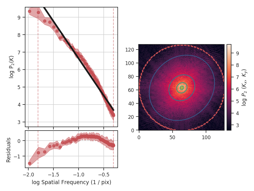
The code returns a summary of the one-dimensional fit and a figure showing the one-dimensional spectrum and model on the left, and the two-dimensional power-spectrum on the right. If fit_2D=True is set in run (the default setting), the contours on the two-dimensional power-spectrum are the fit using an elliptical power-law model. We will discuss the models in more detail below. The dashed red lines (or contours) on both plots are the limits of the data used in the fits. See the PowerSpectrum tutorial for a discussion of the two-dimensional fitting.
The VCA power spectrum from this simulated data cube is \(-4.25\pm0.08\), which is steeper than the power spectrum we found using the zeroth moment (PowerSpectrum tutorial). However, as was the case for the power-spectrum of the zeroth moment, there are deviations from a single power-law on small scales due to the inertial range in the simulation. The spatial frequencies used in the fit can be limited by setting low_cut and high_cut. The inputs should have frequency units in pixels, angle, or physical units. In this case, we will limit the fitting between frequencies of 0.02 / pix and 0.1 / pix (where the conversion to pixel scales in the simulation is just 1 / freq):
>>> vca.run(verbose=True, xunit=u.pix**-1, low_cut=0.02 / u.pix,
...         high_cut=0.1 / u.pix)
                            OLS Regression Results
==============================================================================
Dep. Variable:                      y   R-squared:                       0.985
Model:                            OLS   Adj. R-squared:                  0.984
Method:                 Least Squares   F-statistic:                     866.6
Date:                Thu, 20 Jul 2017   Prob (F-statistic):           2.77e-13
Time:                        15:28:29   Log-Likelihood:                 17.850
No. Observations:                  15   AIC:                            -31.70
Df Residuals:                      13   BIC:                            -30.28
Df Model:                           1
Covariance Type:            nonrobust
==============================================================================
                 coef    std err          t      P>|t|      [0.025      0.975]
------------------------------------------------------------------------------
const          3.7695      0.134     28.031      0.000       3.479       4.060
x1            -3.0768      0.105    -29.438      0.000      -3.303      -2.851
==============================================================================
Omnibus:                        1.873   Durbin-Watson:                   2.409
Prob(Omnibus):                  0.392   Jarque-Bera (JB):                1.252
Skew:                          -0.684   Prob(JB):                        0.535
Kurtosis:                       2.641   Cond. No.                         13.5
==============================================================================
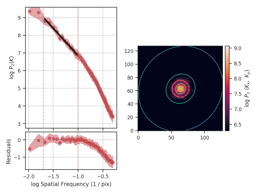
With the fit limited to the valid region, we find a shallower slope of \(-3.1\pm0.1\) and a better fit to the model. low_cut and high_cut can also be given as spatial frequencies in angular units (e.g., u.deg**-1). When a distance is given, the low_cut and high_cut can also be given in physical frequency units (e.g., u.pc**-1).
This example has used the default ordinary least-squares fitting. A weighted least-squares can be enabled with weighted_fit=True (this cannot be used for the segmented model described below).
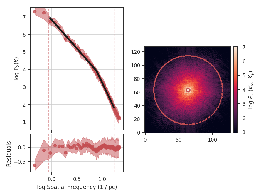
Breaks in the power-law behaviour in observations (and higher-resolution simulations) can result from differences in the physical processes dominating at those scales. To capture this behaviour, VCA can be passed a break point to enable fitting with a segmented linear model (Lm_Seg; see the description given in the PowerSpectrum tutorial). The 2D fitting is disabled for this section as it does handle fitting break points. In this example, we will assume a distance of 250 pc in order to show the power spectrum in physical units:
>>> vca = VCA(cube, distance=250 * u.pc)
>>> vca.run(verbose=True, xunit=u.pc**-1, low_cut=0.02 / u.pix,
...         high_cut=0.4 / u.pix, fit_kwargs=dict(brk=0.1 / u.pix),
...         fit_2D=False)
                            OLS Regression Results
==============================================================================
Dep. Variable:                      y   R-squared:                       0.998
Model:                            OLS   Adj. R-squared:                  0.998
Method:                 Least Squares   F-statistic:                 1.113e+04
Date:                Thu, 20 Jul 2017   Prob (F-statistic):           2.66e-90
Time:                        16:19:33   Log-Likelihood:                 101.91
No. Observations:                  71   AIC:                            -195.8
Df Residuals:                      67   BIC:                            -186.8
Df Model:                           3
Covariance Type:            nonrobust
==============================================================================
                 coef    std err          t      P>|t|      [0.025      0.975]
------------------------------------------------------------------------------
const          3.6333      0.053     68.784      0.000       3.528       3.739
x1            -3.1814      0.047    -67.916      0.000      -3.275      -3.088
x2            -2.4558      0.094    -26.152      0.000      -2.643      -2.268
x3            -0.0097      0.027     -0.355      0.724      -0.065       0.045
==============================================================================
Omnibus:                        8.205   Durbin-Watson:                   1.148
Prob(Omnibus):                  0.017   Jarque-Bera (JB):                7.707
Skew:                          -0.772   Prob(JB):                       0.0212
Kurtosis:                       3.469   Cond. No.                         20.8
==============================================================================

By incorporating the break, we find a better quality fit to this portion of the power-spectrum. We also find that the slope before the break (i.e., in the inertial range), the slope is consistent with the slope from the zeroth moment (PowerSpectrum tutorial). The break point was moved significantly from the initial guess, which we had set to the upper limit of the inertial range:
>>> vca.brk
<Quantity 0.1624771454997838 1 / pix>
>>> vca.brk_err
<Quantity 0.010241094948585336 1 / pix>
From the figure, this is where the curve deviates from the power-law on small scales. With our assigned distance, the break point corresponds to a physical scale of:
>>> vca._physical_size / vca.brk.value
<Quantity 0.14082499334584425 pc>
vca._physical_size is the spatial size of one pixel (assuming the spatial dimensions have square pixels in the celestial frame).
The values of the slope after the break point (x2) in the fit description is defined relative to the first slope. Its actual slope would then be the sum of x1 and x2. The slopes and their uncertainties can be accessed through:
>>> vca.slope
array([-3.18143757, -5.63724147])
>>> vca.slope_err
array([ 0.04684344,  0.104939  ])
The slope above the break point is within the uncertainty of the slope we found in the second example (\(-3.1\pm0.1\)). The uncertainty we find here is nearly half of the previous one since more points have been used in this fit.
The Lazarian & Pogosyan theory predicts that the VCA power-spectrum depends on the size of the velocity slices in the data cube (e.g., Stanimirovic & Lazarian 2001). VCA allows for the velocity channel thickness to be changed with channel_width. This runs a routine that down-samples the spectral dimension to match the given channel width. We can re-run VCA on this data with a channel width of \(\sim 400\) m / s, and compare to the original slope:
>>> vca_thicker_channel = VCA(cube, distance=250 * u.pc,
...                           channel_width=400 * u.m / u.s,
...                           downsample_kwargs=dict(method='downsample'))
>>> vca_thicker.run(verbose=True, xunit=u.pc**-1, low_cut=0.02 / u.pix,
...                 high_cut=0.4 / u.pix,
...                 fit_kwargs=dict(brk=0.1 / u.pix), fit_2D=False)
                       OLS Regression Results
==============================================================================
Dep. Variable:                      y   R-squared:                       0.998
Model:                            OLS   Adj. R-squared:                  0.998
Method:                 Least Squares   F-statistic:                     9739.
Date:                Thu, 20 Jul 2017   Prob (F-statistic):           2.29e-88
Time:                        19:00:25   Log-Likelihood:                 94.310
No. Observations:                  71   AIC:                            -180.6
Df Residuals:                      67   BIC:                            -171.6
Df Model:                           3
Covariance Type:            nonrobust
==============================================================================
                 coef    std err          t      P>|t|      [0.025      0.975]
------------------------------------------------------------------------------
const          1.4422      0.057     25.516      0.000       1.329       1.555
x1            -3.2388      0.051    -64.014      0.000      -3.340      -3.138
x2            -2.8668      0.108    -26.651      0.000      -3.081      -2.652
x3             0.0116      0.030      0.385      0.702      -0.049       0.072
==============================================================================
Omnibus:                        7.262   Durbin-Watson:                   1.043
Prob(Omnibus):                  0.026   Jarque-Bera (JB):                6.646
Skew:                          -0.720   Prob(JB):                       0.0361
Kurtosis:                       3.418   Cond. No.                         20.9
==============================================================================
With the original spectral resolution, the slope in the inertial range was already consistent with the “thickest slice” case, the zeroth moment. The slope here remains consistent with the zeroth moment power-spectrum, so for this data set of \(^{13}{\rm CO}\), there is no evolution in the spectrum with channel size.
An alternative method to change the channel width can be used by specifying downsample_kwargs=dict(method='regrid'). The spectral axis of the cube is smoothed with a Gaussian kernel and down-sampled by interpolating to a new spectral axis with width channel_width (see the spectral-cube documentation).
Constraints on the azimuthal angles used to compute the one-dimensional power-spectrum can also be given:
>>> vca = VCA(cube)
>>> vca.run(verbose=True, xunit=u.pix**-1, low_cut=0.02 / u.pix,
...         high_cut=0.1 / u.pix,
...         radial_pspec_kwargs={"theta_0": 1.13 * u.rad, "delta_theta": 40 * u.deg})
                            OLS Regression Results
==============================================================================
Dep. Variable:                      y   R-squared:                       0.958
Model:                            OLS   Adj. R-squared:                  0.955
Method:                 Least Squares   F-statistic:                     298.9
Date:                Fri, 29 Sep 2017   Prob (F-statistic):           2.36e-10
Time:                        14:57:53   Log-Likelihood:                 11.566
No. Observations:                  15   AIC:                            -19.13
Df Residuals:                      13   BIC:                            -17.71
Df Model:                           1
Covariance Type:            nonrobust
==============================================================================
                 coef    std err          t      P>|t|      [0.025      0.975]
------------------------------------------------------------------------------
const          4.2111      0.204     20.597      0.000       3.769       4.653
x1            -2.7475      0.159    -17.290      0.000      -3.091      -2.404
==============================================================================
Omnibus:                       18.967   Durbin-Watson:                   2.608
Prob(Omnibus):                  0.000   Jarque-Bera (JB):               18.398
Skew:                          -1.869   Prob(JB):                     0.000101
Kurtosis:                       6.932   Cond. No.                         13.5
==============================================================================
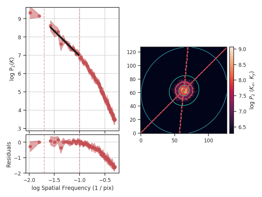
The azimuthal limits now appear as contours on the two-dimensional power-spectrum in the figure. See the PowerSpectrum tutorial for more information on giving azimuthal constraints.
If strong emission continues to the edge of the map (and the map does not have periodic boundaries), ringing in the FFT can introduce a cross pattern in the 2D power-spectrum. This effect and the use of apodizing kernels to taper the data is covered here.
Most observational data will be smoothed over the beam size, which will steepen the power spectrum on small scales. To account for this, the 2D power spectrum can be divided by the beam response. This is demonstrated here for spatial power-spectra.